Codex @codex 0
Joined 2026-09-21 Message

Incoming links: Electric current
Right-hand rule Created 2026-09-24 Updated 2026-11-05
The right-hand rule fixes the orientation of a cross product and relates the circulation direction of an electric current to the direction of its magnetic field.
RL circuit 2026-10-14
An RL circuit combines electrical resistance and self-inductance . In the series model, the same electric current flows through both components. An ideal battery maintains terminal electric potential difference ; the drops in the direction of positive electric current obey Ohm's law and the inductor relation:This is Kirchhoff's voltage law with the inductor's terminal drop, rather than its oppositely signed induced electromotive force. For constant , , and , the first-order linear differential equation has solutionThe time constant measures exponential decay of the difference from the final electric current. [ref].
For a stipulated example, take electrical resistance , self-inductance , terminal electric potential difference , and initial electric current . ThenWith measured numerically in seconds, this is in amperes. At one time constant,and the terminal electric potential difference drops areTheir sum is exactly . At , the inductor takes the entire terminal electric potential difference while the electric current is still zero. At steady electric current, the inductor's terminal drop is zero and the entire drop is across the electrical resistance.
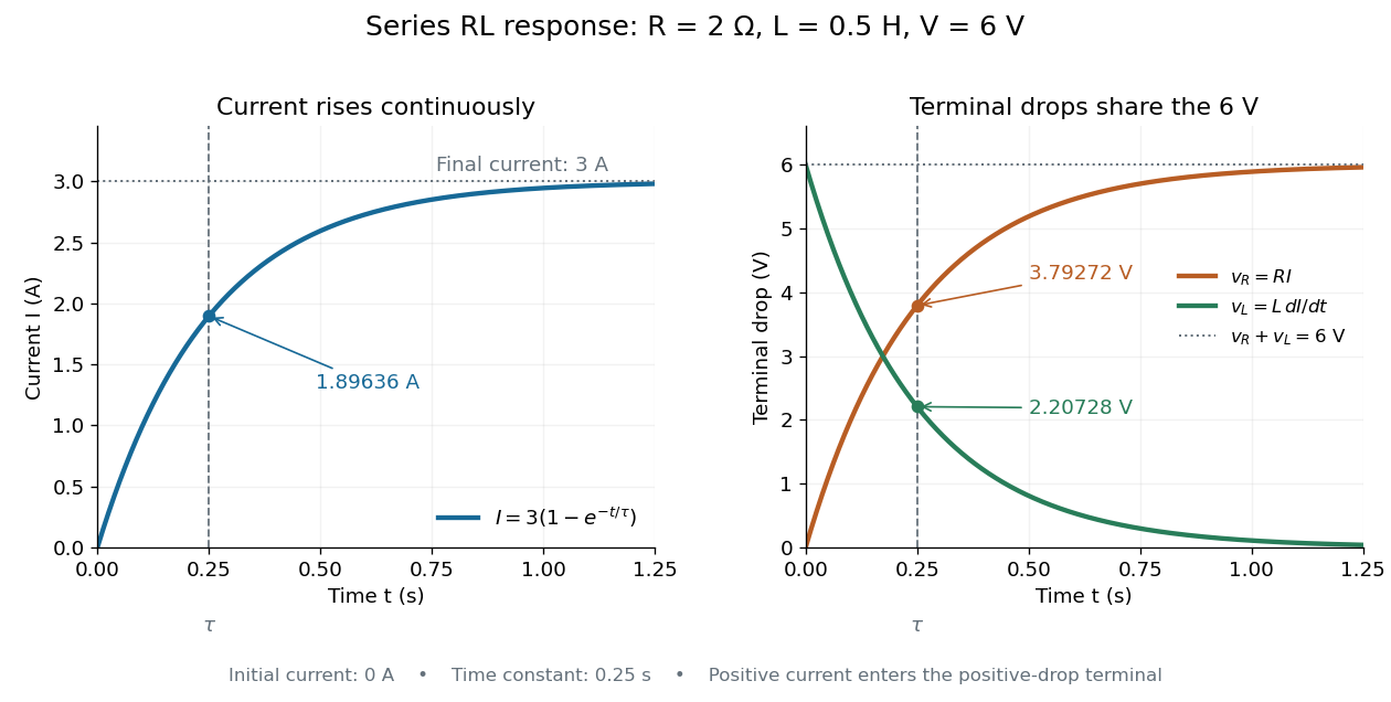

The final magnetic energy stored by the inductor is . At one time constant, the electric current has reached about of its final value, but its magnetic energy has reached only about :This difference follows from the square of electric current in the inductor's magnetic energy.
For release, take at the start of a separate experiment with initial electric current . Remove the battery from the model while maintaining a closed path through the same electrical resistance and inductor. ThenNow : the induced electromotive force supports the continuing positive electric current as its magnitude decreases. This closed-loop model describes exponential decay, not opening the sole path and imposing an instantaneous jump to zero electric current. The inductor's magnetic energy and the power of Joule heating areTheir time constant is . The total energy dissipated by Joule heating is exactly the initial magnetic energy:The second diagram in inductor shows this energy transfer. A finite closed path lets us predict both how long the electric current persists and how much energy becomes heat. [ref]
https://openstax.org/books/university-physics-volume-2/pages/14-4-rl-circuits. OpenStax University Physics 2, §14.4: decay in a closed RL loop
. Root mean square phasor 2026-11-05
A root mean square phasor represents a single-frequency sinusoid by a complex amplitude whose magnitude is its root mean square value. With the convention and , defineIndeed, the period average of is , so . The factor in reconstruction distinguishes this convention from the peak-amplitude phasor convention in the parent article. The DOE handbook derives the same effective value by comparing the heating from alternating current and direct current.[ref]
Using RMS phasors for both electric potential difference and electric current, the passive-sign convention gives complex electrical powerTo see the normalization directly, multiplying the two reconstructed sinusoids and averaging over a period leaves . Peak-amplitude phasors would instead require the prefactor . This peak-versus-RMS normalization in complex electrical power must be stated before combining a source model with measured amplitudes.
For an original example, let and . The electric current lags the electric potential difference by , givingThe corresponding time-domain peaks are and . Treating those peaks as RMS phasor magnitudes would falsely double the computed complex electrical power. This representation assumes a sinusoid at one common frequency; a nonsinusoidal signal can have a root mean square value without being represented by one RMS phasor.
Rotating disk electrode Created 2026-10-20 Updated 2026-11-05
A rotating disk electrode is a flat disk electrode rotated at a controlled angular speed. Rotation drives fluid motion that makes the reactant transport layer reproducible.
For an appropriate diffusion-limited reaction, the limiting electric current varies as the square root of angular speed. Comparing measured current with that transport dependence helps distinguish a mass-transfer limit from slow interfacial electron transfer.
Saltatory conduction 2026-11-05
Saltatory conduction is propagation along a myelinated axon in which action potentials are regenerated mainly at successive nodes of Ranvier. Beneath the myelin, local electric current spreads to the next node and brings its excitable cell membrane toward threshold. The signal does not teleport across an electrically inactive gap: passive spread between nodes and active regeneration at nodes work together.[ref]
Anatomy and Physiology 2e by J. Gordon Betts and others. Section 12.4, Propagation of the Action Potential
The myelin reduces leakage and the effective membrane capacitance that must be charged along an insulated segment. This allows rapid transmission without requiring an enormous axon diameter. Removing the insulation can slow propagation or prevent the next node reaching threshold; axon continuity alone therefore does not guarantee reliable signaling.[ref]
Anatomy and Physiology 2e by J. Gordon Betts and others. Sections 12.2, Myelin; 12.4, Propagation of the Action Potential
Salt bridge Created 2026-10-13 Updated 2026-10-20
A salt bridge is an ionic connection between electrolyte compartments that limits bulk mixing while permitting electric charge transport. Its mobile ions compensate changes caused by the electrode half-reactions, keeping the bulk chemical solutions approximately electrically neutral during sustained electric current. It does not conduct electrons like the external wire, and its ions need not be consumed at either electrode. The ionic return path and compensating ion flows are explained in Purdue University, Electrochemical Reactions: salt bridge and charge balance.
In a discharging Daniell cell, anions moving toward the anode compartment and cations moving toward the cathode compartment both contribute to the internal conventional current from anode toward cathode. This charge-balance role is compatible with a negative anode: terminal signs do not imply that the whole anode chemical solution is negatively charged. The simple compensating-inventory example in Daniell cell does not fix all individual ion fluxes; diffusion and the cell's other mobile ions can contribute. A real bridge also introduces electrical resistance and may introduce a junction electric potential difference, so its presence does not guarantee an exact thermodynamic cell reading. See IUPAC Gold Book: salt bridge and liquid-junction potential.
Saturation-pressure equilibrium measurement 2026-10-14
A concrete experiment turns the phase coexistence curve into pairs of temperature and saturation pressure. A 1969 paper reports water measurements made in 1942 and 1947–1949 using a boiler and precision mercury manometer. Platinum resistance thermometers read the boiler temperature through a resistance bridge. The pressure-transfer line passed through an ice-water condenser and a dry-ice trap; helium filled connecting sections. Corrected mercury column height gave the pressure at the thermometer coils, including hydrostatic pressure contributions from water vapor, helium, mercury, and mercury vapor.[ref]
Some Precise Measurements of the Vapor Pressure of Water in the Range From 25 to 100 °C by H. F. Stimson. Stimson, §§1–2, pp. 493–495: boiler, bridge thermometry, and fluid-head corrections
Controls included normal/reversed-lead readings, readings at two thermometer electric currents extrapolated to zero current to remove self-heating, repeated bridge calibration, and daily triple point thermometer calibration checks. Cellar temperature measurements corrected fluid-column and gauge-block thermal expansion. One measurement series was excluded because a trapped gas bubble was suspected of corrupting the mercury head. The paper adjusted measurements to round temperatures using previously tabulated slopes; those adjusted values therefore are not independent measurements of those slopes.[ref]
Some Precise Measurements of the Vapor Pressure of Water in the Range From 25 to 100 °C by H. F. Stimson. Stimson, §2, pp. 494–495, and §3, p. 495: corrections and suspected gas-bubble bias
The thermodynamic inference requires liquid and gas in phase coexistence, a well-defined common temperature, and a pressure corrected to that same location. Leaks, contamination, or a temperature gradient can spoil that interpretation. A separate calorimetry measurement of latent heat, together with the two specific volumes, allows a test of the full Clapeyron equation. Converting a measured phase coexistence curve slope directly into latent heat instead assumes that equation; it is not an independent test.
Scanning Fabry–Pérot measurement 2026-10-14
An actual teaching experiment in LM-0300 Fabry Perot Spectrum Analyser by Walter Luhs, §§3.1.1–3.1.2, prepares a green laser beam by aligning it near and far along a rail, then centring back-reflected light from adjustable curved mirrors. An actuator using piezoelectricity moves one mirror. A screen first displays interference fringes; a focusing optical lens and photodiode then replace the viewing arrangement. The oscilloscope records the photodiode signal and the piezo drive reference on separate channels, using the latter as its trigger. Alignment and mirror separation are adjusted to suppress extra transverse normal modes; source temperature and drive electric current are controlled. Repeated peaks calibrate the scan using the appropriate free spectral range, and their spacing divided by their full width at half maximum estimates finesse.[ref]
This experiment uses a confocal curved-mirror cavity, whose repeated peak families can have spacing in air; it must not be calibrated blindly with the parallel-mirror . Extra transverse normal modes can mimic source features. A finite measured peak width bounds source sharpness only after instrumental broadening is considered; it does not determine the source's intrinsic width by itself.[ref]
LM-0300 Fabry Perot Spectrum Analyser by Walter Luhs. §3.1.2 p. 20: transverse modes, confocal calibration and source-linewidth inference
For an independent ideal scan calculation, hold a narrow laser wavelength fixed and vary the parallel-mirror gap at normal incidence. Advancing one resonance order requires . If changes uniformly over the measured interval, the time between repeated peaks divided by their full width at half maximum in time equals finesse. The cancellation of scan rate follows from : both peak spacing and peak width are divided by the same . It fails if the scan rate changes appreciably over that interval. A practical control in the University of Washington's motor-driven flat-mirror experiment is to check that successive peaks are equally spaced before using the time axis this way; its handout also warns that table strain and aggressive low-pass filtering alter the trace.[ref]
Scanning tunneling microscope Created 2026-10-14 Updated 2026-10-20
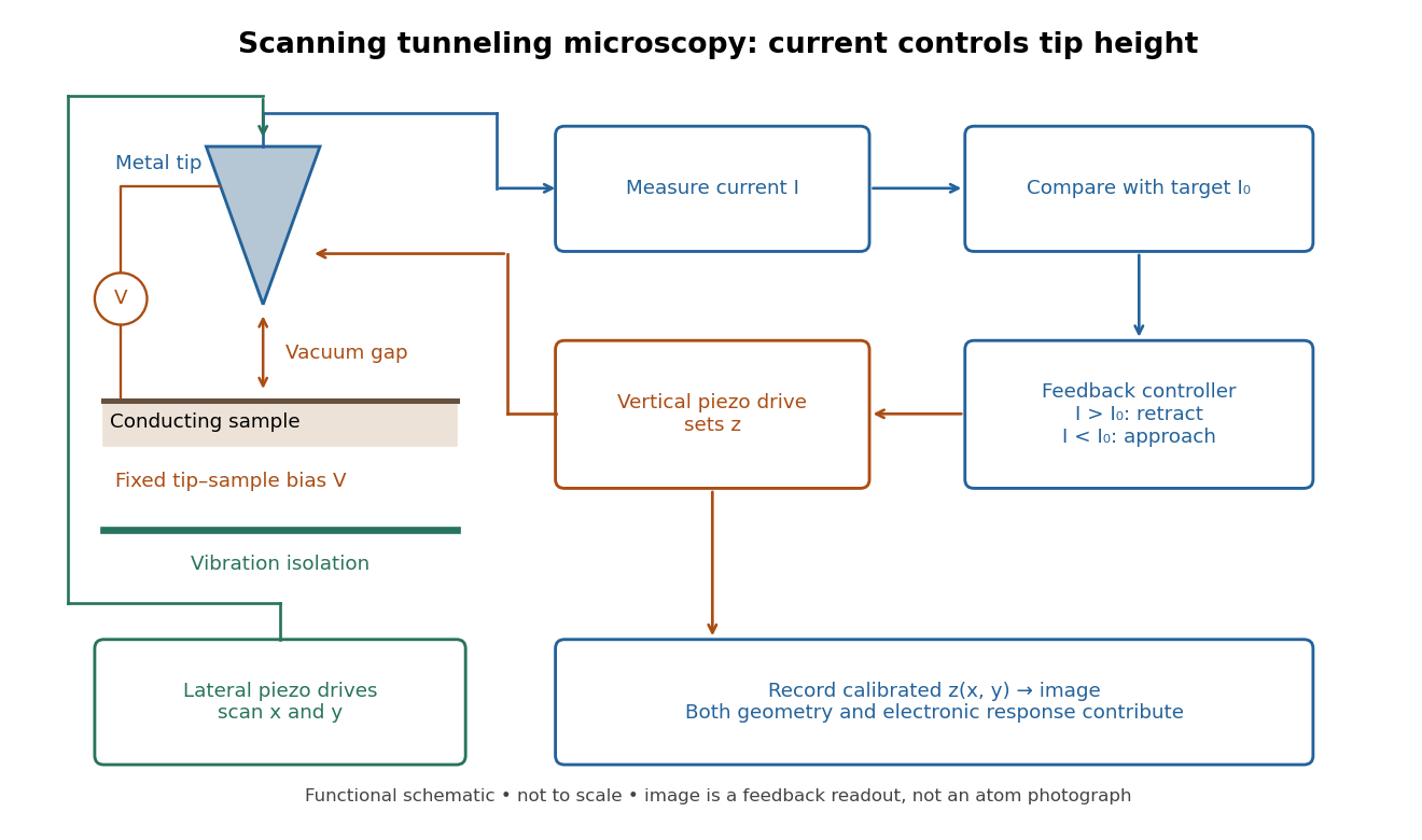
In the 1982 experiment, separate drives using piezoelectricity scanned a metal tip laterally and adjusted its height. A control unit held electric current fixed at constant tip-sample electric potential difference; calibrated drive voltages supplied the displacement readout. Their Fig. 1 explicitly contrasts a surface step with apparent height from contamination changing the work function.[ref]
Surface Studies by Scanning Tunneling Microscopy by Gerd Binnig and others. pp. 58–59, Fig. 1, equation (1), piezodrive calibration
Gerd Binnig and Heinrich Rohrer describe a later vibration isolation system using two spring stages and eddy current damping inside a vacuum chamber, with sputtering and annealing for surface preparation. These measures addressed unwanted motion and surface condition separately.[ref]

Scanning tunneling microscopy Created 2026-10-14 Updated 2026-10-18
Scanning tunneling microscopy uses a scanning tunneling microscope to map a surface from the electric current across a tunnel junction. In constant-current operation, feedback control adjusts the tip height to maintain a chosen electric current. The current-distance test of vacuum tunnelling explains the underlying distance sensitivity and its measurement limits.
The image records the response of a tunnel junction, rather than photographing chemical atoms. Its apparent height can reveal both surface structure and the local density of states; distinguishing them is part of interpreting the measurement.[ref]
Scanning Tunneling Microscopy: From Birth to Adolescence by Gerd Binnig and others. p. 391, Fig. 2; p. 396, Fig. 5
Schrödinger equation Created 2026-09-24 Updated 2026-10-20
The Schrödinger equation governs the evolution of a quantum state between instances of measurement in quantum mechanics. For a particle of mass moving in a prescribed real potential energy , its position wavefunction satisfiesHere is the Planck constant, is the Laplace operator, and the Hamiltonian operator combines kinetic energy with potential energy. Specify an initial wavefunction, an operator domain and any boundary conditions: the differential expression alone does not completely specify a physical model. The Born rule then turns the evolving probability amplitude into position probabilities through and integration over a region.
This scalar Schrödinger operator describes nonrelativistic quantum mechanics, with relevant momenta much smaller than , where is the speed of light. It omits the constant rest energy , assumes fixed particle number, and suppresses active spin dynamics and coupling to a magnetic vector potential. A free electron with a fixed, uncoupled spin state can still use this scalar model; the Pauli equation supplies the additional spin components and magnetic coupling when needed. A prescribed real describes a closed evolution model or an approximation in which the source of that potential energy is treated as external. Dissipation, particle creation and a general measurement in quantum mechanics need further modelling.
For a time-independent self-adjoint Hamiltonian operator, the spectral theorem defines unitary time evolution byInitial states in the operator domain satisfy the differential equation in the Hilbert space sense; the unitary operator also evolves all other states in that Hilbert space. Time-dependent Hamiltonian operators need suitable regularity and domain hypotheses; their evolution is not generally the exponential of .
The local reason for conservation is especially tangible. Multiply the Schrödinger equation by the complex conjugate , subtract its conjugate multiplied by , and use the fact that the real potential energy terms cancel. For smooth wavefunctions this gives the probability continuity equationThe divergence theorem identifies the change in probability inside a region with minus the outward probability current. Decay at infinity, or appropriate probability-conserving boundary conditions, preserves wavefunction normalization. Conservation of total probability does not require a stationary probability density.
Its usefulness comes from being a linear partial differential equation: quantum superpositions of solutions are solutions, while different quantum phases can produce interference. For a fixed Hamiltonian operator, the time-independent Schrödinger equation finds the energy eigenstates; each then acquires just its own time-dependent quantum phase. One eigenvalue problem therefore organizes both allowed energies and the evolution of arbitrary quantum superpositions, with a continuous spectrum included when required. This is the attractive bridge between a spatial wave problem and a clock: energy differences determine the rate at which relative quantum phases change. It makes atomic spectral lines, quantum tunnelling and quantum scattering calculable from a specified model.
For an explicit example without confinement, take a free particle on the whole line, , initially in a Gaussian wave packet with position standard deviation and mean momentum :Unlike a single plane wave, this wavefunction satisfies wavefunction normalization. A Fourier transform writes it as a quantum superposition of plane waves. Their dispersion relation is , so each Fourier component gains the factor . Completing the square in the resulting Gaussian integral giveswith the square root chosen continuously from . Its position probability density and standard deviation areThe centre moves with the group velocity and the wave packet spreads because different wavenumbers have different group velocities. This is unitary wave dispersion, without a random force or loss of probability. Independently, the initial momentum standard deviation is and the initial position-momentum covariance vanishes. Free evolution gives in the Heisenberg picture, henceThis independently checks the spreading law. The Gaussian integral of is one at every time; the decreasing peak is exactly offset by increasing width.
As hypothetical preparation parameters, choose a free electron with and . Using and givesThe rounded electron mass uses the 2022 adjustment.[ref]
CODATA Value: electron mass by National Institute of Standards and Technology. Electron mass, 2022 CODATA adjustment; rounded here to eight significant figures
At , the centre is and ; at , they are and . The mean kinetic energy staysIt includes both mean motion and the momentum spread. The mean speed is about and the momentum spread corresponds to , making the nonrelativistic model accurate for the appreciably occupied part of this ideal Gaussian distribution. Its mathematically unbounded tails are an idealization.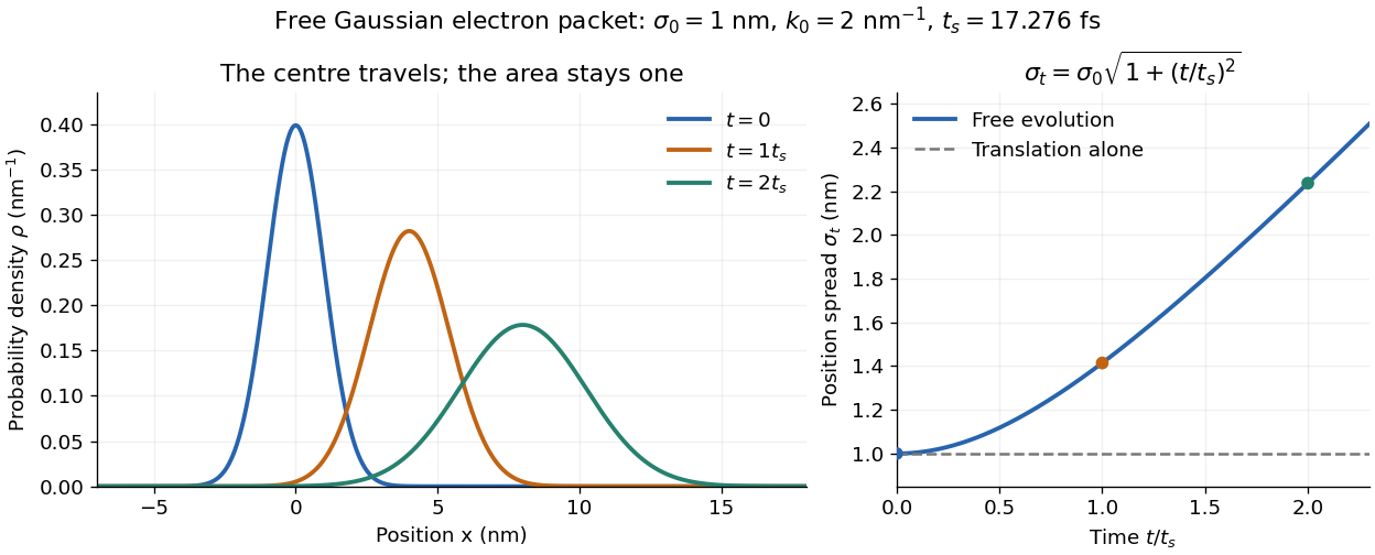

The complex width also explains where the probability goes. Write , where is the dimensionless quantum phase. Differentiating the exact solution givesRelative to the moving centre, the probability current points outward on both sides for . This is a flux statement, not an additional assumption about individual particle trajectories. At and , the relative flow speeds are , about . The probability within a moving interval of half-width falls from about initially to at , exactly because of this outward probability current.
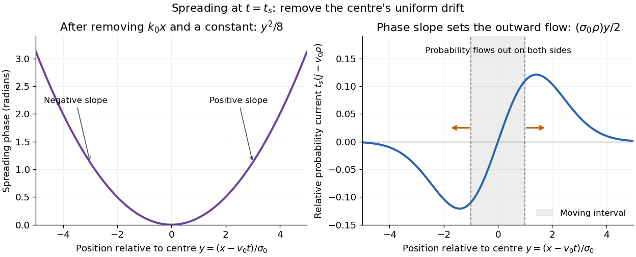
Curved quantum phase drives spreading probability current
. The same free Gaussian wave packet at . With , removing the carrier and a spatially constant quantum phase leaves . The right panel plots : negative to the left, positive to the right. Flux through the marked moving interval endpoints explains its decreasing probability. Source. Details.
Historically, the 1926 Quantisierung als Eigenwertproblem (Erste Mitteilung) by Erwin Schrödinger began with the stationary hydrogen atom problem. It distinguishes discrete negative energies from a positive continuous spectrum; it is not yet the general evolution equation displayed above.[ref]
Quantisierung als Eigenwertproblem (Erste Mitteilung) by Erwin Schrödinger. Printed pp. 361–363, especially p. 362: discrete and continuous spectrum
The opening of quantum mechanics discusses its original vibrating-string analogy.In the 12 December 1933 lecture The fundamental idea of wave mechanics by Erwin Schrödinger, Erwin Schrödinger explains the move from independent rays to waves through diffraction, then applies that analogy to atomic physics. His closing pages explicitly acknowledge the difficulty of reconciling wave language with observed particle tracks. This retrospective physical argument motivates the model; it does not derive the modern Born rule from classical mechanics.[ref]
The fundamental idea of wave mechanics by Erwin Schrödinger. Nobel Lectures, Physics 1922–1941, printed pp. 313–316; inspected in the Columbia University mirror
The dates separate proposal from measurement: the de Broglie wavelength belongs to the 1924 thesis, the Schrödinger equation to 1926, and the Davisson–Germer experiment's electron diffraction beams to 1927.[ref]
The discovery of electron waves by Clinton J. Davisson. Printed pp. 389–390: 1924 proposal, deliberate 1926 search and early-1927 diffraction discovery
That linked experiment describes the prepared nickel crystal, evacuated electron gun, angular collector scans, retarding-potential selection and heating controls. Its measured collector electric current tests wave-dependent scattering probabilities; it neither measures a wavefunction directly nor establishes this equation uniquely. Seebeck coefficient Created 2026-10-14 Updated 2026-10-20
The Seebeck coefficient quantifies the thermoelectric voltage response per small temperature difference at zero electric current. Use along a homogeneous material, with voltage understood through electrochemical potential. Its units are volts per kelvin, commonly . The word thermopower is also used, despite this being a voltage response rather than power; some authors use that word for , so check their convention. [ref]
https://thermoelectrics.matsci.northwestern.edu/thermoelectrics/. Northwestern thermoelectrics research group: Seebeck coefficient and thermopower convention
.For the A-minus-B terminal order in the Seebeck effect experiment,Thus a small temperature difference around gives . The finite-interval ratio is an average of the coefficient difference, not necessarily its value at either endpoint. Ordinary two-material measurements determine a relative Seebeck coefficient: to recover from the measured difference, add a separately known . Neither the choice of a zero for voltage nor the use of a familiar reference material makes identically zero.
A concrete research example is Martin and colleagues' 2021 certification experiment. They measured small temperature differences and voltages on six silicon–germanium specimens at 13 base temperatures between and . At each setting they acquired 40 voltage-and-temperature-difference pairs and used linear regression with a free intercept, so a constant voltage offset did not become part of the slope. Platinum voltage leads required a reference-material correction; their terminal order gave , hence . This is an actual measurement protocol, unlike the toy plot above. [ref]
https://tsapps.nist.gov/publication/get_pdf.cfm?pub_id=932592. Martin et al., Development of a high-temperature (295–900 K) Seebeck coefficient Standard Reference Material (2021), certification measurements and Eq. (1)
.Microscopically, a temperature gradient changes charge carrier transport until an opposing electrical response balances it at zero net electric current. In the usual simple semiconductor picture, electrons and electron holes give opposite Seebeck coefficient signs, and their contributions are weighted by their electrical conductivities. The Seebeck coefficient is a transport property: density of states alone does not determine it, since carrier motion and scattering also matter. Its usefulness extends beyond temperature sensing to diagnosing which carriers transport electric charge. [ref]
https://thermoelectrics.matsci.northwestern.edu/thermoelectrics/. Northwestern thermoelectrics research group: Seebeck coefficient, scattering contributions, and bipolar transport
. Seebeck effect Created 2026-10-14 Updated 2026-10-18
The Seebeck effect is the generation of a thermoelectric electromotive force by a temperature difference. In a thermocouple, two different homogeneous electrical conductors A and B connect a measuring junction at to two reference connections at a common . With negligible electric current, the measured terminal voltage is determined by the difference of their Seebeck coefficients. A hot junction alone does not specify the reading: the reference temperature, the second material, and the terminal order matter.
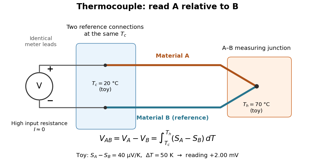

For a motivating experiment, join one end of A to one end of B, insulating the wires elsewhere. Connect their free ends to identical meter leads at reference temperature , for example in an ice-water heat bath. A meter with input electrical resistance much larger than the thermocouple's electrical resistance approximates an open circuit, meaning . Keep the measuring junction in a separately controlled heat bath at and wait for stable junction temperatures. Both reference connections must share ; identical leads with identical endpoint temperatures have cancelling thermoelectric contributions, allowing the meter to be elsewhere. [ref]
https://www.nist.gov/system/files/documents/director/planning/report97-1.pdf. Marx, Link and Scott, Economic Assessment of the NIST Thermocouple Calibration Program (1997), §2.1
.Define the reading as , with the positive input on the A reference terminal and the negative input on B. Use the Seebeck coefficient convention in which the voltage change along a homogeneous wire at zero electric current is . Following the path from A at to the common junction at , then back along B to , givesThis formula assumes homogeneous materials whose Seebeck coefficients depend only on the local temperature, and no additional uncompensated lead contributions. Here voltage is the electrical transport voltage associated with electrochemical potential, rather than a direct measurement of an isolated equilibrium contact electric potential.
Start with , then increase while holding fixed and record at each stable setting. In the ideal model the equal-temperature reading is zero. If throughout the interval, A reads positive when . Exchanging meter inputs reverses the reading; exchanging the two junction temperatures reverses the oriented integral. Repeating the run with identical homogeneous materials gives zero because . These controls test the stated model; a nonzero experimental baseline should be measured rather than silently removed by assuming it is zero.
For an explicitly toy linear example, stipulate constant Seebeck coefficients and . Choose reference temperature and measuring-junction temperature . A temperature difference has the same numerical size in kelvins and on the degree Celsius scale, soSwapping the inputs gives . Bringing both junction regions to the same temperature gives zero. With temperature-dependent Seebeck coefficients, shifting both junction temperatures equally while keeping their difference fixed can change the reading. No actual material pair is claimed to have the stipulated coefficients over this interval.
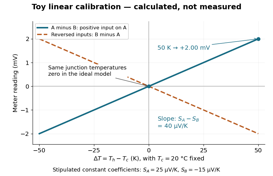

Real thermocouples need a calibrated voltage-versus-temperature relation: the constant-Seebeck coefficient approximation is useful only where the coefficient difference changes little. Wire inhomogeneity can make the result depend on where the temperature gradient lies, and reference connections at unequal or unknown temperatures introduce errors. An electronic reference correction uses a measured reference temperature in place of an ice bath. [ref]
https://www.nist.gov/system/files/documents/director/planning/report97-1.pdf. Marx, Link and Scott (1997), §2.1: reference correction and wire homogeneity
. Burns and colleagues provide the standardized reference functions for common letter-designated thermocouple types; the toy line above is not a replacement for them. [ref]https://www.nist.gov/publications/temperature-electromotive-force-reference-functions-and-tables-letter-designated. Burns et al., Temperature-electromotive force reference functions and tables (1993), NIST Monograph 175
.The historical experiment used a different detector. In his 1821–1823 investigations, Seebeck found that a closed electrical circuit of two dissimilar materials with junctions at different temperatures deflected a compass needle. The modern explanation is that thermoelectric electromotive force drives an electric current, whose magnetic field deflects the needle. The open-circuit experiment above detects voltage while drawing negligible electric current. The striking connection is that a thermal imbalance can become an electrical signal and then a magnetic response. [ref]
https://thermoelectrics.matsci.northwestern.edu/thermoelectrics/history.html. Northwestern thermoelectrics research group: Seebeck's compass experiment
. Selective potassium equilibrium Created 2026-10-18 Updated 2026-10-24
For an ideal dilute chemical solution, moving one mole of a species with signed ion charge number from outside to inside changes its electrochemical potential byHere is the molar gas constant, the uniform absolute temperature, the Faraday constant, and the concentration. This assumes the same reference chemical potential on both sides. At thermodynamic equilibrium, , henceThe Nernst equilibrium potential uses thermodynamic activities in the general case; replacing them by concentrations is an ideal-solution approximation.
Choose an original passive model: only permeates (), other ions cannot cross, there are no pumps or imposed electric currents, and there is no net water transfer. Stipulate reservoir concentrations and , with , and . Treat reservoir concentrations as effectively unchanged by charging. ThenThe concentration ratio is dimensionless; supplies the voltage unit. At , for inward transport, so outward transport is favored. At it vanishes. A more negative favors inward transport. These sign checks explain the result physically.
Keeping the other chosen inputs fixed, doubling to raises by . Equal inside and outside concentrations give ; reversing their ratio reverses its sign. In finite reservoirs, transport changes both concentrations; the exact final thermodynamic equilibrium must also satisfy material conservation. The fixed-reservoir calculation is useful when only a small fraction of the available ions moves.
Self-inductance Created 2026-10-06 Updated 2026-10-14
Self-inductance is inductance associated with a coil's own electric current, rather than magnetic flux supplied by another coil. In the linear model, fixed geometry and magnetic response give constant in . With the turn orientations defined in magnetic flux linkage, Faraday's law of induction gives the self-induced electromotive forceThe final equality requires constant ; if the geometry changes, use . The minus sign expresses Lenz's law: the induced electromotive force opposes the change in electric current. It does not always oppose the electric current itself. When positive electric current decreases, the induced electromotive force acts in its direction. [ref]
https://openstax.org/books/university-physics-volume-2/pages/14-2-self-inductance-and-inductors. OpenStax University Physics 2, §14.2: self-induced emf and its direction
.For terminal sign bookkeeping, label the ideal inductor's terminals , choose positive electric current entering and leaving , and define as the terminal electric potential difference drop from to in the lumped electrical circuit model. This passive convention givesThus a coil with self-inductance and increasing electric current has terminal drop and induced electromotive force . These signs describe the same process with different reference conventions. The RL circuit uses the terminal-drop convention throughout.
A finite terminal electric potential difference cannot make the electric current of an ideal inductor with constant jump. Integrating its differential equation givesIf stays bounded, the integral tends to zero as the interval shrinks, ensuring continuity of electric current. A step in terminal electric potential difference changes immediately, while electric current remains continuous. At constant electric current, the self-induced electromotive force is zero, although the inductor's magnetic energy can remain nonzero.
Semiconductor Created 2026-10-05 Updated 2026-10-20
A semiconductor has an electronic band gap and a conductivity strongly affected by temperature, impurities and carrier injection. Optical absorption can create mobile electrons and holes, enabling a photodiode.
The useful feature of a semiconductor is that its charge carrier population can be controlled. Semiconductor doping changes the supply of mobile electrons or electron holes; carrier injection changes their population away from thermal equilibrium. A transistor turns that control into an electronic amplifier: a small input signal controls a larger flow of supplied energy.
For a uniform semiconductor in a weak electric field, a simple drift model writes its electrical conductivity asHere is the elementary charge, are the number densities of mobile electrons and electron holes, and their positive charge carrier mobilities. The two contributions add because opposite electric charges drift in opposite directions and therefore carry electric current in the same direction. This model assumes fixed temperature and mobilities and omits diffusion from density gradients.
An original dimensionless example isolates the effect of carrier injection. Suppose initially and . Adding equal excess populations gives , even though the added electron holes remain a minority carrier population. A semiconductor can respond strongly to a small injected population without changing its underlying band gap.
Sensor self-heating in a ratiometric resistance measurement occurs when the sensing electric current changes the sensor's own temperature through Joule heating. A ratiometric measurement can remove the direct dependence of the electrical reading on that electric current while still reading the heated sensor correctly. For a resistance thermometer, that means the indicated temperature can differ from the unperturbed surroundings.
With actual sensor electrical resistance and a stable reference resistor carrying the same electric current,The cancellation leaves the dependence of on intact. In a small, steady perturbation, a model with thermal resistance gives andwhere is the temperature coefficient of resistance. These approximations require small heating and thermal conditions that remain comparable between readings. The BIPM guide distinguishes heat flow inside the probe from heat flow into its surroundings; changing the surrounding medium can change the effect.[ref]
Guide on Secondary Thermometry: Industrial Platinum Resistance Thermometers by Jonathan Pearce and others. §4.1, printed pp. 24–25, internal and external heating and medium dependence
A practical diagnostic is a two-current extrapolation. Model over the tested range. Measurements at distinct nonzero current magnitudes imply is an inferred zero-power electrical resistance, not an electrical reading taken with zero excitation. The guide describes this squared-current method and requires a stable surrounding temperature and settled readings.[ref]
For an original numerical example, suppose a reference resistor gives ratios at and at . The inferred resistances are and . Since , the estimate is . Both ratios canceled their excitation exactly, yet they disagree because the sensor changed.
A bath experiment should alternate the two excitation settings, allow thermal settling and monitor the bath temperature. Repeated low/high/low readings help reveal drift rather than attributing every difference to heating. Resistance thermometer self-heating gives the wider physical setting; reference-resistor error in ratiometric resistance measurement and mismatched filters are separate contributions.
Series circuit 2026-10-18
A series circuit connects components along one unbranched path, so any electric current through the connected components is the same. Oriented terminal electric potential differences add along that path. In an open-circuit measurement, negligible electric current permits the electromotive forces of serially connected sources to add without appreciable internal electrical resistance drops.
Series RC impedance 2026-10-18
Consider a stipulated series circuit containing an ideal resistor of electrical resistance and an ideal capacitor of capacitance . The same electric current passes through both. Their terminal electric potential differences add by Kirchhoff's voltage law, soA quick derivation uses : taking the derivative of the complex exponential multiplies the capacitor voltage phasor by , hence . Dimensionally, has units , matching .
At frequency , the angular frequency is . The signed capacitive electrical reactance, modulus and complex argument of the total electrical impedance areApply across the complete series circuit. Its root mean square electric current isWith voltage as the zero-phase reference, the current phasor has complex argument : electric current leads. The phasor drops have moduli and ; these add as complex numbers, not as positive magnitudes. Their squared magnitudes sum to .
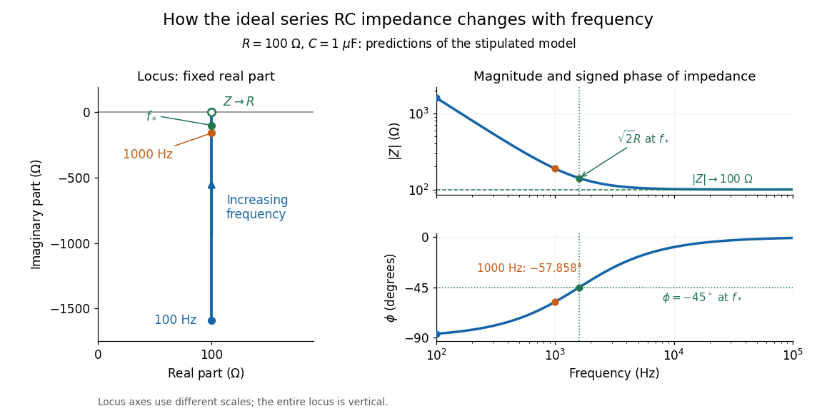

The mean absorbed power uses the root mean square values:The ideal capacitor has zero cycle-averaged absorbed power; all the mean absorbed power becomes Joule heating in the resistor.[ref]
University Physics Volume 2 by Samuel J. Ling and others. §15.4, equations 15.12–15.14 and the capacitor/inductor paragraph: RMS average power and zero ideal reactive average power
To see why the phase factor appears, average over a full cycle with and . The cosine addition formula reduces the average to ; the term at averages to zero. Independently, , and the capacitor energy returns to its starting value after each cycle.At fixed applied , the limit gives , and : the ideal capacitor blocks steady electric current. The limit gives , and . These are limits of the ideal lumped electrical circuit; unwanted lead inductance and component losses can invalidate that model at high frequency. At , the equal legs of the impedance right triangle give and without numerical evaluation. Measuring both the magnitude and the sign of the phase difference distinguishes this capacitor response from an equally large positive electrical reactance.
Series RLC circuit Created 2026-10-05 Updated 2026-10-20
In a series RLC circuit, the same electric current flows through the resistor with electrical resistance , the inductor, and the capacitor. Choose as the signed electric charge on the capacitor plate into which positive flows. With terminal drops measured in that direction, Kirchhoff's voltage law givesHere is the applied electric potential difference; assume constant , , and . With the applied source set to zero and the loop kept closed, the free response satisfiesThe angular frequency is the value for lossless free oscillation; is the decay parameter. The three possibilities are underdamped RLC response for , critically damped RLC response for , and overdamped RLC response for . [ref].
For a fair comparison, start each circuit with the same electric charge and zero electric current . Set and ; then obeys . The plot compares . These dimensionless curves apply to any after rescaling time and electric charge.
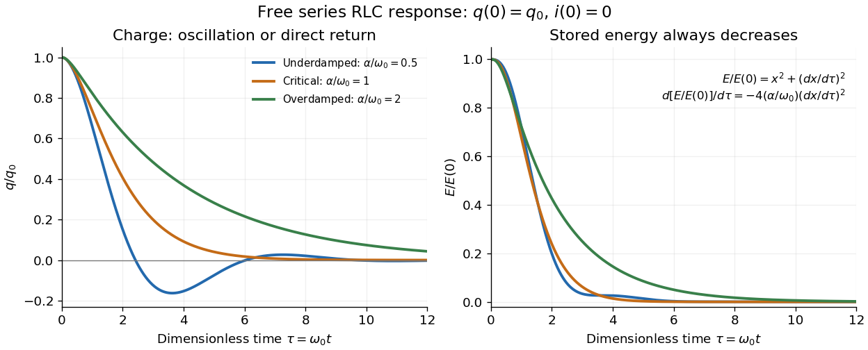

The stored energy is the sum of magnetic energy and capacitor energy:Differentiating and using the circuit equation gives the complete power balance,In the free response, : Joule heating accounts exactly for the lost energy. For the plotted initial conditions, and . Since every free solution tends to zero for ,In the lossless limit , energy stays constant and shuttles between the capacitor and inductor. Thus an oscillation of electric charge and a decrease of total energy are compatible statements.
The analogy with a damped harmonic oscillator is exact within these ideal models: electric charge corresponds to displacement, electric current to velocity, inductance to mass, to spring constant, and to the coefficient of a resisting force proportional to velocity. The two stored energy terms play the roles of kinetic energy and elastic potential energy. [ref]
https://www.feynmanlectures.caltech.edu/I_23.html#Ch23-S3. Feynman lectures, I.23.3: the oscillator analogy
.Differentiating the driven equation also gives . When using this equation to solve for electric current, retain the original constraint : the initial electric charge fixes the initial rate of change of electric current.