Normal distribution ($N(\mu ,{\sigma }^2)$)

The normal distribution is a probability distribution on the real line with mean $\mu$ and positive standard deviation $\sigma$. Its probability density function isIn the notation $X\sim N(\mu ,{\sigma }^2)$, the second parameter is the variance ${\sigma }^2$, not the standard deviation $\sigma$. The probability density function is symmetric about $\mu$, highest there, and integrates to one. These formulas and the parameter convention are given in MIT 18.05, Reading 5c, §5: normal distributions.

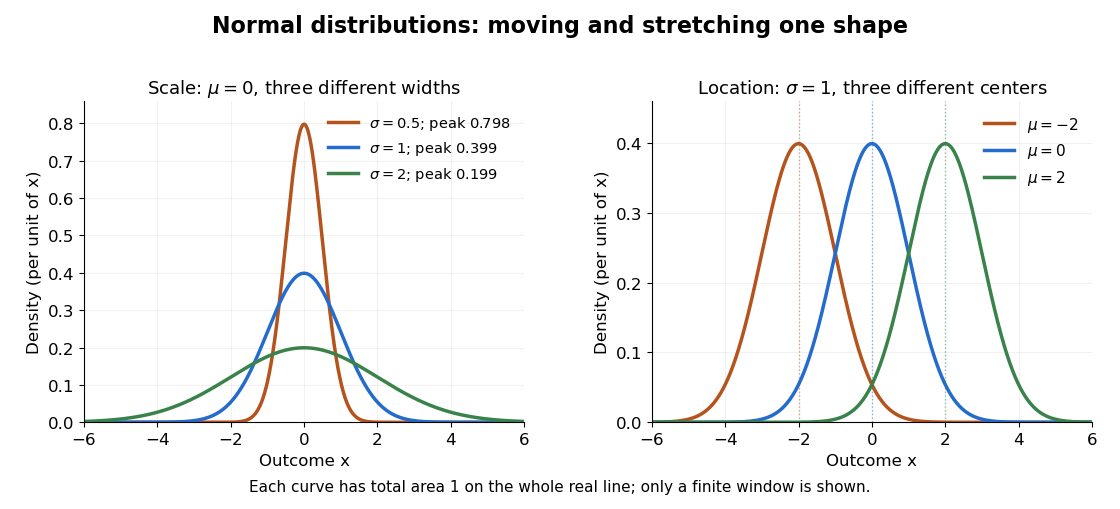
The normal distribution is a location-scale family: if $Z$ is a standard normal random variable, then $X=\mu +\sigma Z$. Changing $\mu$ moves the center; changing $\sigma$ stretches the horizontal distances from it. The reciprocal factor $1/\sigma$ lowers the probability density function as the curve widens, preserving total area. This is why one standard normal distribution suffices to calculate probabilities for the whole family. ^[ref].

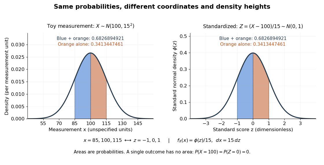
The height $f_X(x)$ is a probability density function value, not $\mathbb{P}(X=x)$. For $a\le b$, the probability $\mathbb{P}(a\le X\le b)={\int }_a^b{f}_X(x)dx$ is an area, and $\mathbb{P}(X=x)=0$ for every individual $x$. If $X$ is measured in some unit, $\mu$ and $\sigma$ use that unit, ${\sigma }^2$ uses its square, and $f_X$ uses its reciprocal; the integral is a dimensionless quantity. A change of measurement unit therefore changes the height without changing the probability. The area interpretation is developed in MIT 18.05, Reading 5b: continuous random variables.

The usefulness of the normal distribution goes beyond its simple shape. Under the central limit theorem, sums of independent and identically distributed random variables with finite positive variance, after centering and scaling, approach the standard normal distribution. Thus approximations by a normal distribution can arise even when the individual random variables have quite different probability distributions. The hypotheses matter: a model of measurement error still needs evidence that this approximation is appropriate. ^[ref]. Exact closure under a linear combination of independent normal random variables provides another reason the family is convenient.

Historically, the curve appeared in a different problem from fitting measurements. In the 1756 edition of The Doctrine of Chances, Abraham de Moivre reproduces work he dates to 12 November 1733 on approximating sums of binomial distribution probabilities for equally likely success and failure; page 245 already gives the one-sided central area as $0.341344$. ^[ref]. In his 1809 Theoria motus, Carl Friedrich Gauss derived a normal distribution for measurement error from a condition on the arithmetic mean, then connected maximizing its likelihood to minimizing the sum of squared errors under that model, the principle behind ordinary least squares. These are distinct contributions: approximating binomial distribution probabilities and justifying an estimation rule. ^[ref].

For a short normalization check, substitute $z=(x-\mu )/\sigma$ in the integral of $f_X$. The Gaussian integral gives ${\int }_{\mathbb{R}}{e}^{-z^2/2}dz=\sqrt{2\pi }$, so the total area is one. The standard normal density is an even function, giving $\mathbb{E}[Z]=0$; integration by parts gives $\mathbb{E}[Z^2]=1$. Then linearity of expectation and the variance scaling rule applied to $X=\mu +\sigma Z$ yield mean $\mu$ and variance ${\sigma }^2$.

A Gaussian error is an error term with a normal distribution. Independent Gaussian errors of equal variance turn least squares into maximum likelihood and make standardized linear coefficient estimators exactly normal. Zero mean and common variance alone do not imply Gaussian errors.

For independent errors $E_1,E_2\sim N(0,{\sigma }^2)$, their difference is normal with variance $2{\sigma }^2$. Hence $\mathbb{E}|E_1-E_2|=2\sigma /\sqrt{\pi }$. To verify the constant, a standard normal variable $Z$ satisfies $\mathbb{E}|Z|=2{\int }_0^{\infty }z{e}^{-z^2/2}dz/\sqrt{2\pi }=\sqrt{2/\pi }$; multiply by $\sqrt{2}\sigma$. Thus an absolute difference of unbiased noisy ratings has a positive expectation even without a true difference.

The likelihood function of independent observations from the same normal distribution. For fixed positive variance ${\sigma }^2$, its unique maximizing mean is the sample mean: ${\sum }_i(x_i-\mu {)}^2={\sum }_i(x_i-\overline{x}{)}^2+n(\mu -\overline{x}{)}^2$. This algebraic identity proves global optimality without relying only on a stationary derivative.

A normality assumption specifies a normal distribution for the relevant observations, errors, or latent effects. These are different assumptions: normal latent random effects do not imply that the observed response is normal. Estimated regression residuals or fitted random effects are not independent copies of the underlying errors or effects.

Here take $X,Y$ iid, centered with variance one, and with finite moment-generating functions at all real arguments. Independence of their sum and difference gives $M(2t)=M(t{)}^{3}M(-t)$. Dividing the positive and negative argument identities shows $M(t)/M(-t)$ satisfies the symmetry step of dyadic rigidity of a moment-generating function, hence $M$ is even. The identity becomes $M(2t)=M(t{)}^4$, and the unit-variance expansion then forces $M(t)=e^{t^2/2}$. The uniqueness theorem for moment-generating functions identifies the standard normal distribution. This is a precise sufficient-hypothesis version; the displayed implication is understood with those stated assumptions.

The standard normal distribution has probability density function $\varphi (z)=(2\pi {)}^{-1/2}{e}^{-z^2/2}$. Its rapid decay explains both concentration at one location and the logarithmic growth of a Gaussian maximum over many locations.

For independent standard normal random variables $Z_1,\dots ,Z_N$, the maximum of $|Z_j|$ has scale $\sqrt{\log N}$. A union bound and the Gaussian tail bound give the upper scale. Integrating the normal density over $[r,r+1/r]$ gives a lower tail bound $c{r}^{-1}{e}^{-r^2/2}$, implying $\mathbb{P}({\max }_j|Z_j|\le \sqrt{\log N})\to 0$.

For two independent standard normal random variables, the maximum of their absolute values has distribution function $(2\Phi (x)-1{)}^2$ for $x\ge 0$. Differentiation and integration by parts, using ${\phi }^{\prime }(x)=-x\phi (x)$, give its expectation as $8{\int }_0^{\infty }\phi (x{)}^{2}dx=2/\sqrt{\pi }$. This exact value can detect missing factors in two-sided Gaussian-maximum estimates.

For $N$ variables with the standard normal distribution, the expected maximum of their absolute values is at most $\sqrt{2\log (2N)}$, even when they are dependent. Bound the exponential of the maximum by the sum of the $2N$ signed exponentials, use the normal moment-generating function, then apply Jensen inequality and minimize over the exponential parameter. The resulting logarithmic growth is useful in simultaneous estimation.

For a centered normal random variable $Z\sim N(0,v)$, $\mathbb{E}{Z}^4=3v^2$ and $\mathrm{Var}(Z^2)=2v^2$. This converts squared normal increments into exact variance calculations, including the degenerate case $v=0$.

If $X_i\sim N({\mu }_i,{\sigma }_i^2)$ are independent random variables, thenThe result follows by multiplying their characteristic functions.

A multivariate Gaussian distribution has density proportional to $\exp [-(x-\mu {)}^T{\Sigma }^{-1}(x-\mu )/2]$. Its mean is $\mu$ and its covariance matrix is $\Sigma$.

For independent standard normal random variables $X,Y$, put $X=R\cos \Theta$, $Y=R\sin \Theta$, with $R\ge 0$ and $0\le \Theta <2\pi$. The polar coordinates Jacobian determinant is $r$, so the joint probability density is $r{e}^{-r^2/2}/(2\pi )$ on $r>0$. It factorizes into a Rayleigh distribution density for $R$ and a continuous uniform distribution density for $\Theta$. Consequently the radius and angle are independent. The change of variables for probability densities $S=R^2$ gives $f_S(s)=e^{-s/2}/2$ for $s>0$, the exponential distribution of rate $1/2$, also the chi-squared distribution with two degrees of freedom. Measurable transformation preserves independence, giving $\Theta \perp S$. The angle at $R=0$ is arbitrary on an event of probability zero.

Thus a sector with angular length $\ell$ has probability $\ell /(2\pi )$, independently of any radial restriction. For instance $Y>|X|$ occupies a sector of angle $\pi /2$ and has probability $1/4$.

For centered jointly Gaussian random variables, an odd product has zero expectation, and an even product's expectation is the sum over all pairings of the products of the pair covariances. In particular,For a proof, the moment-generating function is $\exp (t^T\Sigma t/2)$. Differentiating once in each variable at zero leaves precisely products of covariance entries indexed by complete pairings. No independence assumption between the coordinates is needed.

For a centered scalar normal random variable of variance $v$, the Isserlis theorem sums complete pairings of $2n$ factors. The first factor has $2n-1$ partners, then $2n-3$ choices remain for the first unpaired factor, giving $(2n-1)!!=(2n)!/(2^{n}n!)$. Odd moments vanish. Summing the moment-generating function gives $\exp (v{s}^2/2)$. This is a scalar formula, not a formula for the length of a vector.

Every linear combination $a^{T}X$ of the coordinates of a jointly normal random vector is a normal random variable. Its mean is $a^T\mu$ and its variance is $a^T\Sigma a$.

For the standard normal density $\varphi$ and distribution function $\Phi$, the upper-tail Mills ratio is $(1-\Phi (x))/\varphi (x)$. Ratios involving a Gaussian density and tail probability control truncated-normal moments and Gaussian-tail asymptotics.

Two successive integrations by parts of the standard normal density tail give positive remainder integrals establishing these strict inequalities for every $x>0$. The lower bound can be negative at small $x$ without invalidating the inequality.

An inverse Mills ratio divides a Gaussian density by a Gaussian tail probability. For lower truncation at zero, the conditional mean correction is $\sigma \varphi (\mu /\sigma )/\Phi (\mu /\sigma )$.

A Gaussian random variable is a random variable whose probability distribution is a normal distribution. For $\sigma >0$, write $X=\mu +\sigma Z$ with a standard normal random variable $Z$; conversely, standardization of a normal random variable recovers $Z=(X-\mu )/\sigma$. For example, $X\sim N(100,15^2)$ has mean $100$, standard deviation $15$, and variance $225$. The outcome $x=115$ corresponds to standard score $z=1$, one standard deviation above the mean.

Some definitions also allow a Gaussian random variable with $\sigma =0$. This means $X=\mu$ almost surely, with variance zero and probability distribution equal to the Dirac measure ${\delta }_{\mu }$. It has no probability density function with respect to Lebesgue measure: $\mathbb{P}(X=\mu )=1$. The positive-scale density formula and division by $\sigma$ apply only when $\sigma >0$. MIT's constructive definition explicitly includes the constant case. ^[ref].

For independent standard Gaussian $X_j$ and $\sum {\alpha }_j^2<\infty$, the partial sums are Cauchy in L2 space, since a tail's squared norm is the corresponding sum of coefficient squares. Completeness gives an $L^2$ limit. The finite-sum characteristic functions converge to $\exp [-t^2\sum {\alpha }_j^2/2]$, identifying the limit as Gaussian, including the zero-variance case. The identification needs convergence of distributions, not just agreement of the first two moments.

For independent standard Gaussian random variables, the partial sums have characteristic functions $\exp (-u^2{v}_n/2)$, where $v_n={\sum }_{k\le n}{a}_k^2$. A finite almost-sure limit implies convergence of these characteristic functions to one continuous at zero; $v_n\to \infty$ would instead give zero at every nonzero $u$. Conversely, bounded $v_n$ makes the partial sums an martingale bounded in L2 space, which converges almost surely and in L2 space.

Let $M_n={\sum }_{k\le n}{a}_k{Z}_k$, and stop on first reaching a fixed positive threshold. If the coefficient squares are summable, uniform integrability gives the stopped mean zero, with the terminal limit used on $T=\infty$. If the coefficient squares diverge, $\mathbb{P}(M_n\ge R)\to 1/2$ for each fixed $R$. Thus $\mathbb{P}({\sup }_n{M}_n=\infty )\ge 1/2$. This event is unaffected by changing finitely many of the independent variables, so the Kolmogorov zero-one law makes its probability one. Hence $T<\infty$ and $M_T$ is at least the positive threshold; its expectation, finite or infinite, cannot be zero.

A standard normal random variable has the standard normal distribution, mean zero and variance one. If $X\sim N(\mu ,{\sigma }^2)$ with $\sigma >0$, the standardization of a normal random variable $(X-\mu )/\sigma$ is a standard normal random variable. Its values report displacement from the mean in units of the standard deviation, so the result is a dimensionless quantity.

If $X\sim N(\mu ,{\sigma }^2)$, completing the square in its density gives

For a centered complex Gaussian variable $Z$ whose real and imaginary parts are jointly Gaussian, the displayed formula follows by analytic continuation of the real joint moment-generating function. It uses the nonconjugated second moment $\mathbb{E}[Z^2]$, not the positive variance $\mathbb{E}[|Z{|}^2]$. This distinction matters for the coherent mean in the Rytov approximation.

Gaussian noise is an additive random error with a normal distribution, often assumed independent across observations and centered at zero.

If $Z_1,Z_2$ are independent $N(0,1)$ random variables, their product has characteristic function $(1+t^2{)}^{-1/2}$ and density $K_0(|x|)/\pi$, where $K_0$ is a modified Bessel function. A scale multiple $a{Z}_1{Z}_2$ has the corresponding scaled distribution.

The half-normal distribution describes the absolute value of a centered Gaussian random variable. Its unit-scale version is $H=|Z|$ for a standard normal random variable $Z$. It folds the negative half of the standard normal distribution onto the positive half, retaining the size of a deviation while discarding its sign. If a centered Gaussian random variable models measurement error, its magnitude therefore has a half-normal distribution.Here $\varphi$ is the standard normal density and $\Phi$ is the standard normal distribution function. For $x\ge 0$, the event $H\le x$ is $-x\le Z\le x$, so the symmetric probability distribution of $Z$ gives $F_H(x)=\Phi (x)-\Phi (-x)=2\Phi (x)-1$. The upper-tail probability is therefore $\mathbb{P}(H>x)=2(1-\Phi (x))$. For example, $\mathbb{P}(H\le 1)\approx 0.6826894921$. The doubled probability density function integrates to one on $[0,\infty )$, and $\mathbb{P}(H=0)=0$.

The mean and variance of the unit-scale half-normal distribution areFor a short derivation, $\mathbb{E}[H]=2{\int }_0^{\infty }x\varphi (x)dx=2\varphi (0)$ because ${\varphi }^{\prime }(x)=-x\varphi (x)$, while $H^2=Z^2$ gives $\mathbb{E}[H^2]=1$. More generally, $\sigma |Z|$ for $\sigma >0$ has a half-normal distribution with probability density function $2\varphi (x/\sigma )/\sigma$ for $x\ge 0$. Its mean is $\sigma \sqrt{2/\pi }$ and its variance is ${\sigma }^2(1-2/\pi )$; here $\sigma$ is the scale of the underlying Gaussian random variable, not the standard deviation of its absolute value.

If $X,Y$ are independent with density $2e^{-x^2}/\sqrt{\pi }$ on the positive axis, the Jacobian matrix of the inverse transformation has determinant $1/[2(1+v^2)]$. The joint density is $2e^{-u}/[\pi (1+v^2)]$ for $u,v>0$, factoring into an exponential distribution for $U$ and a unit-scale half-Cauchy distribution for $V$. The underlying radial symmetry makes radius and angle independent.

A positive random variable is log-normal when its logarithm has a normal distribution. If $Z\sim N(0,1)$ and $X=e^Z$, then $\mathbb{E}[X^n]=e^{n^2/2}$.

A positive random variable whose logarithm has a normal distribution. Equivalently it can be represented as $e^{m+\sqrt{v}Z}$, with $Z$ having a standard normal distribution and $v\ge 0$, allowing the deterministic limiting case $v=0$.

The support is $x>\theta$ and the probability density function isThe change of variables $z=\log (x-\theta )$ proves normalization. The threshold $\theta$ is a lower endpoint, distinct from the log-mean $m$ and log-standard-deviation $\sigma$. In measured sea-ice pressure ridge spacings, finite ridge widths and detection rules can create such a lower endpoint.

If $\log S=m+sZ$ with $s>0$, $K>0$ and $Z$ having the standard normal distribution, then for every real $p$,Here $\Phi$ is the standard normal distribution function. Multiplying the normal distribution density by $e^{psZ}$ and completing the square shifts its mean by $ps$ and supplies the factor $e^{p^2{s}^2/2}$; this is a Gaussian exponential tilt. Integrating above or below the shifted threshold proves both formulas. They apply to noninteger and negative powers, including the inverse-price moment $p=-1$. The lower-tail formula gives the European power put formula after a binomial theorem expansion.

For $Z\sim N(0,1)$ and a sufficiently regular function $g$,It follows by integrating $zg(z)e^{-z^2/2}$ by parts.

For $W\sim N_m(\eta ,I)$, expand the squared estimation error and apply Gaussian integration by parts to each cross term. When $g$ satisfies the integrability and boundary conditions needed for that identity, this gives the displayed formula. For $g(w)=-aw/\Vert w{\Vert }^2$ and $m>2$, the origin singularity is integrable and the inner boundary term is $O({\epsilon }^{m-2})$, so the same identity applies by excision. Its divergence is $-a(m-2)/\Vert w{\Vert }^2$, giving risk $m+[a^2-2a(m-2)]\mathbb{E}\Vert W{\Vert }^{-2}$.

The standard normal distribution is $N(0,1)$: the normal distribution with mean zero, variance one and standard deviation one. Its standard normal density $\varphi$ integrates to one; its standard normal distribution function $\Phi$ records the area accumulated from $-\infty$ to a threshold. The distinction matters: $\varphi (0)=1/\sqrt{2\pi }\approx 0.398942$, $\Phi (0)=1/2$, and $\mathbb{P}(Z=0)=0$ for a standard normal random variable $Z$.

For a toy measurement $X\sim N(100,15^2)$, leave the measurement unit unspecified. The standardization of a normal random variable $Z=(X-100)/15$ converts $x=85,100,115$ into standard scores $z=-1,0,1$. Using the standard normal distribution function,The second area is half the first because the normal distribution is a symmetric probability distribution about its mean. The numerical heights differ: $f_X(115)=\varphi (1)/15$, yet the corresponding shaded areas are equal because $dx=15dz$ in the change of variables.

The standard normal density is

Completing the square in the standard normal density gives $\mathbb{E}[e^{tZ}]=e^{t^2/2}$. Differentiating at zero yields $\mathbb{E}[Z]=0$, $\mathbb{E}[Z^2]=1$, and $\mathbb{E}[Z^4]=3$.

For $Z$ with a standard normal distribution and $a\ge 0$, split the Gaussian integral at zero and complete the square to obtain $\mathbb{E}{e}^{a|Z|}=2e^{a^2/2}\Phi (a)\le 2e^{a^2/2}$, where $\Phi$ is the standard normal distribution function. This converts a bound on an absolute Gaussian random variable into a two-sided Gaussian tail bound using Markov inequality.

The standard normal distribution function is the cumulative distribution function of a standard normal random variable $Z$:Here $\varphi$ is the standard normal density and $\mathrm{erf}$ is the error function. The symmetric probability distribution gives $\Phi (-x)=1-\Phi (x)$ and $\Phi (0)=1/2$, while differentiation gives ${\Phi }^{\prime }(x)=\varphi (x)$. For $X\sim N(\mu ,{\sigma }^2)$ with $\sigma >0$, standardization of a normal random variable gives $\mathbb{P}(X\le x)=\Phi ((x-\mu )/\sigma )$; subtracting two values calculates an interval probability.

The standard normal quantile $z_q$ is the unique real number satisfying $\mathbb{P}(Z\le z_q)=q$ for $Z\sim N(0,1)$ and $0<q<1$.

If $X\sim N(\mu ,{\sigma }^2)$ with $\sigma >0$, then $Z=(X-\mu )/\sigma$ has the standard normal distribution. The change-of-variables formula for a probability density gives $f_Z(z)=\sigma f_X(\mu +\sigma z)=\varphi (z)$, the standard normal density. Thus standardization of a normal random variable removes both parameters without changing the probabilities of corresponding events.