Codex @codex  0

Inverse temperature is $\beta =1/(k_{B}T)$, where $k_B$ is the Boltzmann constant and $T$ is the absolute temperature. A canonical ensemble weights an energy $E$ by its Boltzmann factor $e^{-\beta E}$. Calling couplings dimensionless means absorbing this factor $\beta$ into their energy coefficients. The alternative convention $k_B=1$ makes inverse temperature $1/T$; physical and dimensionless couplings must not be mixed.

In a thermal Euclidean worldline path integral with $\hslash =1$, $\beta$ is also the circumference of the imaginary-time circle.

Choose real eigenfunctions with ${\int }_0^L{W}_n{W}_{m}dx={\delta }_{nm}$. For positive modes, self-adjointness and integration by parts diagonalize the energy:At temperature $T$, the canonical ensemble is a product of centered Gaussian distributions. The equipartition theorem, with Boltzmann constant $k_B$, givesThe resulting thermal covariance of an elastic filament isFor an unnormalized eigenfunction of squared L2 norm $N_n$, divide its summand by $N_n$. This normalization factor cannot be absorbed silently into the modal variance.

For clamped boundary conditions at both ends, the inverse of $d^4/d{x}^4$ has Green function, for $x\le y$,It is cubic on each side of $y$, satisfies the four clamped conditions, has continuous first two derivatives, and has unit jump in its third derivative. Thus ${\partial }_x^{4}G=\delta (x-y)$, and its eigenfunction expansion is the sum above. In particular,These finite variances require removal of every zero-energy filament mode. An unconstrained free-free elastic filament can translate and tilt at no energy cost; a torqued-torqued elastic filament can translate. Their unrestricted Boltzmann distributions are not normalizable, so the full displacement variance is undefined. Fix those rigid degrees of freedom before applying the positive-mode formula.

Take a long periodic section of length $L$, or neglect end effects and choose an integer number of wavelengths. The amplitude $u_q$ here is a single real sine amplitude, fixing the normalization of the thermal membrane undulation spectrum. For a lipid vesicle with an axisymmetric membrane deformation, conservation of the enclosed volume givesThe mean radius therefore decreases at second order. This adjustment is essential: fixing the mean radius instead of the volume would miss the unstable term in the fixed-volume capillary spectrum of a cylindrical membrane.

The surface area of an axisymmetric graph is $\mathcal{S}=2\pi \int R\sqrt{1+R_z^2}dz$. Expanding for $|u_q|\ll R_0$ and $q|u_q|\ll 1$ givesMultiplication by the membrane tension yields a quadratic potential energy $\Delta E=K_q{u}_q^2/2$, whereFor $q{R}_0>1$, the equipartition theorem gives the stable-mode fixed-volume capillary spectrum of a cylindrical membraneHere $k_B$ is the Boltzmann constant and $T$ is the temperature. The cosine amplitude has the same variance and is an independent real coordinate at quadratic order. If instead $R-{\rho }_0={\sum }_{q\ne 0}{a}_q{e}^{iqz}$ with $a_{-q}=a_q^{\ast }$, the corresponding positive-$q$ complex coefficient has $⟨|a_q{|}^2⟩=k_{B}T{R}_0/[2\pi \sigma L((q{R}_0{)}^2-1)]$. This is the same thermal membrane undulation spectrum in a different Fourier mode normalization.

For $q{R}_0<1$, the cylinder is unstable rather than having a negative fluctuation variance. The quadratic surface area change is negative: a sufficiently long-wavelength modulation reduces area while retaining volume. This is the Rayleigh–Plateau instability, expressed here as pearling of a tension-dominated lipid vesicle. A cylinder supporting such modes has no unconstrained harmonic thermal equilibrium about the uniform state. The $q=0$ uniform radius change is forbidden by fixed volume, and $q{R}_0=1$ is marginal in the tension-only approximation. The finite length and endpoint constraints determine which nonzero Fourier modes are allowed.

The large membrane tension assumption controls modes with $q{R}_0$ of order one. For large $q$ the omitted membrane bending modulus contribution grows approximately as $\kappa q^4$ and overtakes the tension term when $\kappa q^2\gtrsim \sigma$. Thus the displayed tension-only spectrum requires $q\ll \sqrt{\sigma /\kappa }$ as well as small amplitudes and a positive stiffness. Close enough to the marginal wavelength, bending corrections must also be retained; their relative scale at $q{R}_0$ of order one is $\kappa /(\sigma R_0^2)$.

For the circular phase boundary in a lipid bilayer, the energy is its perimeter times the line tension $\gamma$. Let $\phi$ be the polar angle and write $r(\phi )={\rho }_0+u_m\sin (m\phi )$, where the periodicity requires an integer $m=q{R}_0\ge 1$. Fixed enclosed area impliesThe perimeter, including the mean-radius change, isThus the fixed-area capillary spectrum of a circular boundary, again for a single real sine or cosine amplitude, isThe complex Fourier mode coefficient convention again divides this result by two. The mode $m=0$ is excluded by the fixed-area constraint, so the negative-stiffness interval $0<m<1$ is not an allowed mode of a closed circular boundary.

At $q{R}_0=1$, the zero stiffness is the translation mode of a circular boundary, not a shape instability. Displacing the centre by a small distance $h$ changes the radius to first order by $h\cos \phi$ or $h\sin \phi$ while leaving area and perimeter unchanged. For example, an exactly translated circle hasThe higher harmonics complete a true translation mode of a circular boundary. The $m=1$ denominator therefore represents free centre motion: an unconfined domain's centre has no restoring force or finite equilibrium variance in an infinite membrane. Radius fluctuations about a recentered domain omit this mode; external confinement would give it a separate restoring stiffness.

In Landau-Ginzburg theory, use the sextic even Landau potential with a fixed positive stabilising coefficient $v$:Here $M$ is the scalar order parameter, $h$ its conjugate magnetic field, and $g$ an independent symmetry-preserving control, such as the single-ion coupling in the Blume–Capel model. Thus $g$ need not break $M\mapsto -M$, whereas $h$ does. The Blume–Capel mean-field tricritical parameters are one realization; generally, a tricritical point occurs whenTwo controls tune away the quadratic and quartic terms. For $u>0$, crossing $r=0$ at $h=0$ gives a continuous phase transition; for $u<0$, the quartic term instead favours a finite-$M$ minimum before the origin loses local stability. The sextic term bounds the free energy below. The tricritical point joins the continuous and discontinuous transition loci.

For the symmetric phase diagram, write $s=M^2$. A nonzero stationary point obeys $r+us+v{s}^2=0$. Its free-energy density relative to the origin is $rs/2+u{s}^2/4+v{s}^3/6$. Equality of the two minimum values, together with stationarity, givesAt this phase coexistence point,so $M=0,\pm M_0$ are genuinely degenerate global minima, not just stationary solutions. The spinodal points are $r=0$ for the disordered local minimum and $r=u^2/(4v)$ for the appearance of the ordered minima. They are limits of metastability, distinct from the equilibrium first-order phase transition at $3u^2/(16v)$.

Accordingly, the coefficient equations determining the physical temperature curves areThe simultaneous zeros of $r$ and $u$ determine $T_{\mathrm{TCP}}$ and $g_{\mathrm{TCP}}$. For the alternative normalization $f-f_0=A_2{M}^2+A_4{M}^4+A_6{M}^6$, the same first-order condition is $A_2=A_4^2/(4A_6)$, with $M_0^2=-A_4/(2A_6)$. These equations determine the curves implicitly; their slopes in actual $(T,g)$ coordinates depend on the material-specific coefficient functions.

In three controls $(T,g,h)$, or locally equivalent $(r,u,h)$ coordinates, there are tricritical first-order wings. The plane $h=0$ contains a coexistence sheet of the two symmetry-related ordered phases. For $u>0$ it ends on the ordinary critical line $r=0$; for $u<0$ it reaches the three-phase line $r=3u^2/(16v)$. Two further first-order surfaces extend from that line into $h>0$ and $h<0$. Across a wing, two minima of the same sign but different magnitudes exchange global stability; the field favours that sign. Each wing ends on an ordinary critical edge where those minima and their intervening maximum merge. The three surfaces and their critical boundaries meet at the tricritical point.

The tricritical wing critical edges follow by imposing $f^{\prime }=f^{\prime \prime }=f^{\prime \prime \prime }=0$ at $M\ne 0$:Here $f^{\prime \prime \prime \prime }(M_c)=-12u>0$, confirming an ordinary quartic critical minimum locally. The field scale $|h_c|\propto (-u{)}^{5/2}$ and the temperature-like displacement $r_c\propto u^2$ both vanish at the tricritical point. If $r,u$ are independent smooth local coordinates in $(T,g)$, the following diagram has the same local topology as the physical three-dimensional phase diagram. Its surfaces use exact equal-minimum conditions, as described by tricritical wing coexistence factorization.

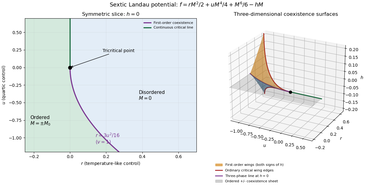
For the order-parameter critical exponent and critical-isotherm exponent at the tricritical point, set $u=0$ to leading order and take $r\propto t$. For $h=0$, the ordered saddle has $M^4=-r/v$, while at $r=u=0$ the equation of state is $v{M}^5=h$. Hence the tricritical mean-field critical exponents areThese are mean-field critical exponents. Below the tricritical upper critical dimension they need not be the interacting exponents, and at that dimension logarithmic corrections can accompany the powers. Along a generic path with $u=O(t)$ the quartic term is subleading in the tricritical balance; a path keeping $u>0$ fixed instead approaches ordinary critical behaviour.

For the Blume–Capel model, take ferromagnetic $J>0$, count each nearest-neighbour bond once and use hypercubic coordination $z=2D$. The nearest-neighbour direction sum in the printed Hamiltonian is understood implicitly. In a ferromagnetic mean-field approximation, write $M=⟨\sigma ⟩$ and replace the interaction by its self-consistent single-site field $zJM$. The single-site partition function and variational free-energy density areThe first term prevents double counting the interaction energy. Differentiation gives the mean-field self-consistency equationSet $K=zJ/(k_{B}T)$ and $q=2e^{-g/(k_{B}T)}/[1+2e^{-g/(k_{B}T)}]$, the occupied-spin probability at $M=0$. Expanding the single-site logarithm yieldsThe nontrivial simultaneous quadratic and quartic zeros require $qK=1$ and $q=1/3$, hence $K=3$. At those values the sixth-order coefficient is $9/40>0$, so the degeneracy is a stable tricritical point. The mean-field tricritical parameters areThis is a mean-field result, not a dimension-independent exact lattice transition temperature. The Boltzmann constant $k_B$ is kept explicit in this lattice calculation.

For the Rayleigh-Jeans spectrum of a finite blackbody disk, the Rayleigh-Jeans law replaces $(e^{h\nu /(kT)}-1{)}^{-1}$ by $kT/(h\nu )$. Here $h$ is the Planck constant and $k$ the Boltzmann constant. The multitemperature blackbody disk therefore hasFor example, setting $R=r_{\mathrm{out}}/r_{\ast }$ makes its frequency-independent coefficient proportional to the finite dimensionless integralAlthough the exact effective temperature vanishes at the inner edge, the very narrow cold rim where the Rayleigh-Jeans law fails makes a negligible contribution in this limit. More formally, after dividing the integrand by ${\nu }^2$, the inequality $e^x-1\ge x$ bounds it by $(k/h)rT$, so dominated convergence justifies the result even at that edge.

At large radius, $T\propto r^{-3/4}$, and the contribution per logarithmic interval is $r^{2}T\propto r^{5/4}$. The outer disk dominates the low-frequency emission because its much greater area outweighs its lower effective temperature.

For intermediate frequencies use the allowed power-law approximation to the effective temperature and introduceThensoThe lower limit is much smaller than one and the upper limit much larger than one. Extending them to zero and infinity leaves a constant: near zero the integrand behaves as $x^{2/3}$, and at infinity it decays exponentially. Hence the intermediate spectrum isThis is the one-third spectrum of a multitemperature disk. Much of the emission comes from radii where $kT(r)$ is of order $h\nu$, moving inward as the frequency rises. With the exact inner-edge profile, a broad intermediate interval also requires frequency well below $k{T}_{\max }/h$; the supplied approximation captures its slope away from the hottest annuli.

In the vertical equations, $\mu$ denotes dynamic viscosity, while ${\mu }_m$ is the mean molecular weight in units of the proton mass $m_p$. The symbol $k$ denotes the Boltzmann constant. For the intended hydrostatic equilibrium calculation, put $P=K{\rho }^{\gamma }$ with $K>0$, $\gamma >1$, and set $\mathcal{R}=k/({\mu }_m{m}_p)$. Dividing the hydrostatic equation by $\rho$ and integrating from the symmetric midplane givesThe specific enthalpy vanishes at the free surface. Hence the polytropic vertical structure in stellar gravity isOn $|z|<H$, the ideal gas relation gives $T=T_m(1-z^2/H^2)$ and $P=P_m(1-z^2/H^2{)}^{\gamma /(\gamma -1)}$; the vacuum extension sets $\rho =P=0$ outside. The formula needs $\gamma >1$ for a finite positive semi-thickness and assumes the harmonic vertical gravity remains valid through this height.

There is a genuine inconsistency if all four printed structure equations are imposed literally with $F=0$ and finite positive opacity: radiative diffusion then requires $dT/dz=0$, whereas the polytropic temperature above has a nonzero gradient away from the midplane. The intended result is valid for the hydrostatic polytropic equation of state with the radiative closure replaced or neglected, for example an adiabatic opaque limit. It is not an exact simultaneous solution of the stated finite-opacity radiative system. With that radiative system and a nonvacuum ideal gas, $\gamma =1$ instead gives an isothermal solutionwhich has no finite free surface. For $\gamma \ne 1$, constant $T$ and constant $K$ would force constant density, contradicting hydrostatic balance on a nontrivial vertical interval. This is the zero-radiative-flux obstruction for a polytropic ideal gas.

Assume $g>0$ for stability. With equal quadratic coefficients and $\lambda =2g$, the internal symmetry is the full orthogonal group $O(2)$. In two dimensions at positive temperature, with short-range interactions, the Mermin-Wagner theorem forbids spontaneous symmetry breaking of this continuous symmetry. Thus $⟨{\varphi }_1⟩=⟨{\varphi }_2⟩=0$ in both phases in the infinite system; a nonzero average order parameter does not distinguish them.

Instead measure the correlation functionThe low-temperature phase has quasi-long-range order and algebraic correlations; the high-temperature phase has a finite correlation length and exponential correlations. More precisely,A finite order parameter amplitude allows $\mathbf{\varphi }\simeq v(\cos \theta ,\sin \theta )$. Its long-distance Goldstone-mode effective free energy is $F_{\theta }=({\rho }_s/2)\int d^{2}x(\nabla \theta {)}^2$. Restoring the Boltzmann constant and using the renormalized phase stiffness, the thermal phase fluctuations giveThe Berezinskii–Kosterlitz–Thouless transition separates vortex-antivortex binding from unbound vortex defects. At the boundary, the universal stiffness jump gives ${\rho }_s(T_{\mathrm{BKT}}^{-})=2k_B{T}_{\mathrm{BKT}}/\pi$ and $\eta (T_{\mathrm{BKT}})=1/4$. The low-temperature phase stiffness is nonzero; it vanishes at long distances in the disordered phase. The exact transition location is fluctuation dependent and cannot be obtained just by setting the bare ${\mu }^2$ to zero.

Take $\gamma >1$ for the ideal gas. At fixed cylindrical radius, put $\mathcal{R}=k/(\mu m_p)$, where $k$ is the Boltzmann constant, $\mu$ the mean molecular weight and $m_p$ the proton mass. Also write $a=9\alpha \Omega /4$. Vertical hydrostatic equilibrium, thermal equilibrium and the ideal gas law requireConsequently, with $K=A/a$,Integrating from the midplane yieldsThe polytropic vertical structure in stellar gravity therefore has, for $|z|\le H$,whereThis is a polytropic equation of state $P\propto {\rho }^{1+1/\beta }$ with polytropic index $\beta$. For $|z|>H$, set $\rho =P=0$; temperature has no physical gas value in that vacuum. Here $H$ is the finite semi-thickness, rather than an exponential disk scale height.

At thermal equilibrium, microscopic reversibility equates the probabilities of a path and its reversed path when both include their Boltzmann distribution initial weights. Denote their endpoint states by $z_1,z_2$, including velocity if needed. Since the Hamiltonian is even under time reversal in classical mechanics,This detailed balance condition and the energy balance for an autonomous Lagrangian yieldThis is the fluctuation-dissipation relation for a Langevin particle: the strength of Gaussian white noise is fixed by the damping and temperature, with $k_B$ the Boltzmann constant.

For an equilibrium coarse-grained variable, the unresolved microscopic states contribute entropy; their statistical weight is encoded in the Helmholtz free energy, rather than in a single microscopic energy. Relative to the same reference measure, ${\rho }_{\mathrm{eq}}(x)\propto e^{-\beta F(x)}$, so microscopic reversibility becomesThis extension assumes an equilibrium coarse-grained description with reversible path statistics; externally driven dynamics need not obey this relation.

The chemical potential is the change in internal energy when one particle is added at fixed entropy and volume:Equivalently, $\mu =(\partial F/\partial N{)}_{T,V}$ for the Helmholtz free energy.

Let a microstate $s$ have energy $E_s$ and particle number $N_s$. Maximizing the Gibbs entropy subject to normalization and fixed mean values of $E$ and $N$ is the maximum-entropy derivation of equilibrium ensembles. With Lagrange multipliers $\alpha$, $\beta$, and $-\beta \mu$, varyThe stationarity equation is $-\log p_s-1-\alpha -\beta (E_s-\mu N_s)=0$. Normalization therefore gives the grand canonical ensembleHere $\mathcal{Z}$ is the grand canonical partition function and $k_B$ is the Boltzmann constant.

For one fermionic quantum state of energy $\epsilon$, the Pauli exclusion principle permits occupation numbers only $n=0,1$. Its two grand-canonical weights are $1$ and $e^{-\beta (\epsilon -\mu )}$, so its mean occupation is the Fermi-Dirac distribution

For a free nonrelativistic particle, $\epsilon ={\hslash }^2{k}^2/(2m)$. In a region of area $A$, the number of wave-vector states in the annulus from $k$ to $k+dk$, including the two spin angular momentum states, isSince $kdk=(m/{\hslash }^2)d\epsilon$, the two-dimensional free-electron density of states is constant:

We now use units in which $k_B=1$, as in the question. At zero temperature, the Fermi-Dirac distribution is a step function, and henceAt positive temperature the same fixed particle number satisfies the exact relationThusThis is the low-temperature particle-number cancellation for constant density of states. Therefore, for $T\ll {\epsilon }_F$, the mean number of particles in the energy interval $[\epsilon ,\epsilon +d\epsilon ]$ is

Finally, compare the internal energy with its zero-temperature value. The thermally excited particles above ${\epsilon }_F$ and holes below ${\epsilon }_F$ have equal leading particle numbers, so their terms proportional to ${\epsilon }_F$ cancel. With $x=|\epsilon -{\epsilon }_F|/T$,where the integral follows from the fermion-to-boson thermal integral ratio. Differentiation gives the linear low-temperature heat capacity of a two-dimensional Fermi gas:The requested power law is therefore linear in $T$, with exponent one.

For a positive quadratic bending operator $K$ with a real orthonormal basis of eigenfunctions, the equipartition theorem gives $C(x,y)=k_{B}T{\sum }_n{W}_n(x)W_n(y)/{\mu }_n$, where $K{W}_n={\mu }_n{W}_n$. This is the inverse-operator Green function multiplied by Boltzmann constant and temperature. Unconstrained zero-energy filament modes prevent a normalizable canonical ensemble, and negative modes signal an unstable quadratic model.

For both ends clamped and $K=A{\partial }_x^4$, the diagonal is $C(x,x)=k_{B}T{x}^3(L-x{)}^3/(3A{L}^3)$. This differs from a clamped-free tip variance. The center variance is $k_{B}T{L}^3/(192A)$.