Diffusion is net transport associated with random microscopic motion. A localized patch of a dilute solute can spread through a stationary solvent: individual molecules move in both directions, but more cross from the crowded side of an imaginary surface than from the less crowded side. This imbalance gives a net diffusive flux down the concentration gradient; the molecules do not need to sense which direction has lower concentration. At uniform concentration, microscopic exchanges continue even though the net diffusive flux vanishes. [ref]
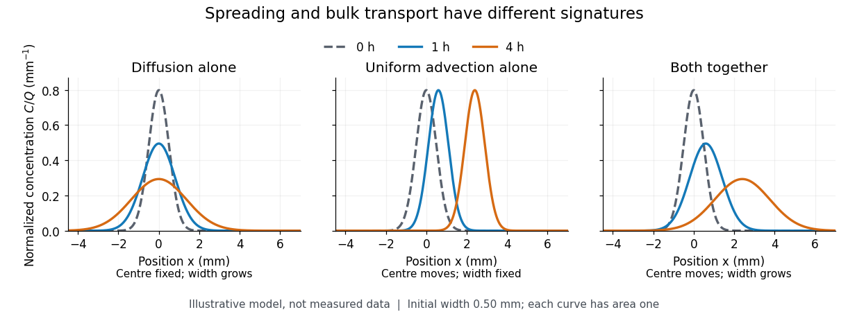
The distinction from advection is easiest to see in a dye patch. Uniform bulk motion carries its centre downstream; diffusion broadens it relative to that centre. Both can happen together. A moving or spreading patch by itself does not identify the mechanism: a nonuniform velocity field can also stretch a patch. [ref]
For a dilute nonreacting solute in a uniform medium at fixed temperature, Fick's first law models the relative diffusive flux as , with scalar diffusion coefficient of units . Here is the amount of substance per unit volume, so has units . With carrier velocity field , the total flux is . The continuity equation, with no sources or chemical reactions, givesFor constant and incompressible flow, this reduces to , where is the Laplacian. In a stationary carrier it is the diffusion equation. These assumptions matter: variable must remain inside the divergence, and changing sources require extra terms. [ref]
https://ocw.mit.edu/courses/1-061-transport-processes-in-the-environment-fall-2008/5536a0bf7f3bd0b21fde2169b93a4b5a_lec_02.pdf. Nepf, MIT: conservation with advective and diffusive fluxes
The useful surprise is the common mathematics: thermal conduction smooths temperature through the analogous heat equation, while molecular diffusion smooths composition. This analogy already motivated the original formulation of Fick's laws. [ref]
https://doi.org/10.1080/14786445508641925. Fick (1855), On liquid diffusion: the analogy with heat conduction
However, the thermal diffusivity and the solutal diffusivity need not be equal. A diffusive time scale means that crossing ten times the distance requires roughly one hundred times the time. This is why molecular diffusion is especially effective across thin layers, and why chaotic advection can assist mixing by making those layers thinner. Physical diffusion is a transport mechanism, distinct from the broader probabilistic class of Markov diffusion.A diffusion tensor describes direction-dependent diffusive flux. In the local, linear Fickian model,where is concentration and the entries of have the units of a diffusion coefficient. A scalar coefficient is recovered when . Material models can instead specify a diagonal matrix or symmetric matrix to represent anisotropic transport.[ref]
Diffusion in solids in the COMSOL 6.4 documentation. Solid, Diffusion: isotropic, diagonal and symmetric diffusion coefficients
For an original two-dimensional example, chooseA concentration gradient directed along , with components , produces diffusive flux in consistent units. The flux need not be antiparallel to the gradient. Nevertheless,for every nonzero gradient in this positive-definite matrix example.
The eigenvectors and have eigenvalues 3 and 1. They identify the principal directions and coefficients. Rotating the coordinate basis changes the matrix entries according to ; it does not change these principal coefficients. In an unbounded, homogeneous, drift-free Gaussian model, displacement covariance is , so spreading also differs along those directions.
Symmetry and positive definiteness are assumptions of this ordinary reciprocal diffusion model, not a definition covering every transport law called a tensor. Boundaries also matter: a reflecting boundary condition constrains , which need not be proportional to the normal derivative alone.
Restricted diffusion is diffusion whose displacement statistics are constrained by boundaries that particles cannot cross. A reflecting boundary condition models an impermeable wall: particles continue moving, but there is no normal diffusive flux through it. Finite permeability would require a different boundary model.
A physical demonstration uses a liquid confined between solid lamellae. In his first-person account, John E. Tanner described constructing 99 mica layers separated by aluminium-foil strips, removing wrinkles and burrs to obtain regular spacing; Edward O. Stejskal inspected the stack with a stereomicroscope. Pulsed magnetic-field gradients encode displacements in the nuclear magnetic resonance signal, allowing motion normal to the barriers to be compared with less confined directions.[ref]
John Tanner, the return to Germelshausen, and the work that nearly never happened by Derek Jones. Printed p.6, mica-stack account and Figure3
This is a material confinement experiment, not a change in the liquid's chemistry.For an original one-dimensional model, let particles diffuse in with constant diffusion coefficient :The wall conditions are homogeneous Neumann boundary conditions for the diffusion equation. Start in equilibrium, so has the uniform distribution on . Its variance isAt long time separation, the positions decorrelate. Consequently the mean squared displacement approachesAt short times relative to , most displacements have not encountered a wall, and the leading scale is the free-diffusion result . For a hypothetical gap , the long-time plateau is and its root is about .
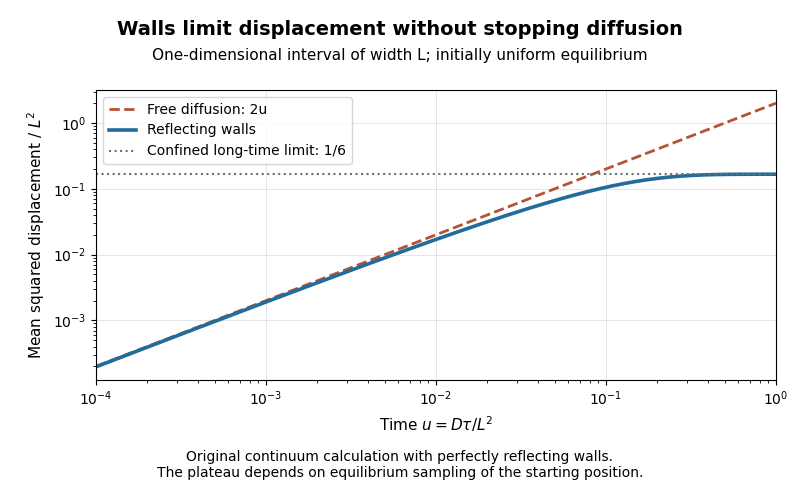
Equilibrium restricted diffusion saturates in a reflecting interval
. Original Neumann-eigenmode calculation with uniform initial positions; time is and mean squared displacement is divided by . Perfectly reflecting walls give a plateau , while free diffusion continues as . These are model curves, not measurements of the mica stack. Details.The initial condition matters: fixing instead gives the long-time value . Likewise, echo attenuation in a confined sample must not automatically be converted into a free-diffusion coefficient. Confinement geometry, timing and the selected boundary model all affect the inference.
A reflecting boundary condition prevents normal particle or probability flux through a wall. For drift-free scalar diffusion with , the condition isHere is the outward unit normal. The last expression is a homogeneous Neumann boundary condition. Integrating the diffusion equation and applying the divergence theorem gives conservation of total probability or material in a closed container.[ref]
Linear Partial Differential Equations Lecture 10 in MIT OpenCourseWare. pp.1–2: diffusive flux, closed container and conserved integral
For an original example, choose units in which the interval is . The densitysatisfies , has zero endpoint derivatives and integrates to one. With , and , its cosine amplitude is about . A nonuniform density therefore relaxes while remaining inside the interval; reflection does not hold the boundary concentration fixed.
For anisotropic diffusion, impose zero normal diffusive flux using the full diffusion tensor. At a wall with , letin consistent units. Then , although . Setting the normal derivative to zero would impose a different condition. Absorption and finite permeability require their own boundary models; a reflecting wall allows continued motion within the available space.
Photon diffusion approximates the spreading of radiation after many scattering events have largely randomized propagation directions. Individual photons travel along paths; their distribution can obey a diffusion equation on scales much larger than a transport mean free path. The longer arrival times arise from longer, repeatedly redirected paths.
For homogeneous, conservative isotropic scattering, the photon diffusion coefficient for isotropic scattering is , where is the transport speed and the scattering mean free path. Directional persistence replaces that scale by a transport mean free path in an appropriate transport model. Crossing a characteristic thickness then takes a time of order , with geometry-dependent factors, which can greatly exceed the direct travel time .
A diffuse photon time-of-flight experiment sends a short pulse into a scattering sample and measures the delayed transmitted or returning light. A pulsed source, a fast photodetector and time-correlated single-photon counting can build an arrival-time histogram from repeated pulses. The detector's timing response must be accounted for before attributing all measured broadening to the sample.[ref]
Time-Correlated Single Photon Counting (technical note v. 2.1) by Michael Wahl. Scattering-medium response measurement and iterative reconvolution, p.3
The 1989 study by M. S. Patterson, Britton Chance and B. C. Wilson used a slab diffusion model to relate picosecond-pulse reflectance and transmittance to absorption and scattering, comparing predictions with preliminary measurements and Monte Carlo simulations.[ref]
Time resolved reflectance and transmittance for the non-invasive measurement of tissue optical properties by M. S. Patterson and others. Abstract: model, optical interaction coefficients and experiment/simulation comparison
The earliest nearly unscattered light, nearby boundaries and strongly directional transport can require a fuller radiative transfer description.A diffuse photon time-of-flight experiment measures the distribution of delays experienced by light traversing a scattering sample. A short-pulse source illuminates the sample; a reference timing signal starts the clock, and a fast photodetector records returning or transmitted photons. Time-correlated single-photon counting accumulates their delays over repeated pulses into a histogram.[ref]
A useful laboratory comparison keeps the source-detector geometry fixed while changing sample thickness or scattering strength. The apparatus needs a defined optical path, a sample holder and the same detection/timing chain for a reference instrument response function. Longer, repeatedly scattered paths broaden the arrival distribution; absorption changes which paths survive to be detected.
Let denote the sample's optical impulse response in the chosen geometry and the normalized instrument response function. A simple model for the expected count-rate trace iswhere denotes convolution, sets the signal scale and represents background counts. Fitting a transport model after including separates sample broadening from instrumental timing spread. A model for an infinite medium cannot simply be substituted for a finite slab's boundary-dependent detector response.
M. S. Patterson, Britton Chance and B. C. Wilson developed analytic slab responses and compared them with preliminary measurements and Monte Carlo simulations in 1989.[ref]
Time resolved reflectance and transmittance for the non-invasive measurement of tissue optical properties by M. S. Patterson and others. Abstract: picosecond pulses, homogeneous-slab model and comparisons
The shape of the delay distribution provides information beyond total transmitted intensity.The counting electronics also matter: if only the first arrival in each pulse period is recorded, multiple arrivals bias the sample toward earlier times. This photon pile-up must be represented or suppressed by the acquisition conditions, rather than mistaken for faster propagation.[ref]
Time-Correlated Single Photon Counting (TCSPC) by PicoQuant. How Does TCSPC Work?: first-photon pile-up and reconstruction of the delay histogram
For conservative photon transport at constant speed , suppose successive scattering directions are independent and isotropically distributed, and free-path lengths follow an exponential distribution of mean . In three spatial dimensions, the resulting long-time diffusion coefficient isHere is the scattering mean free path. These assumptions describe homogeneous, memoryless interactions without absorption.
The velocity autocorrelation function gives a direct derivation. An initially isotropic ensemble has zero mean velocity. During a lag , the probability of no scattering is . No scattering preserves the direction; one or more independent isotropic scattering events give zero expected directional correlation. ConsequentlyThe three-dimensional Green-Kubo formula for diffusion now yieldsThe factor converts the dot-product correlation into one Cartesian component under isotropy.
The same correlation gives the full mean squared displacement:At short times this is ; at long times its leading term is . The model therefore connects direct flights to the diffusive many-scattering limit.
The free-path distribution matters. A fixed-step isotropic random flight with every length equal to has mean-square displacement after steps and elapsed time , giving . Replacing exponential flights by fixed-length flights thus changes the coefficient by a factor of two. For anisotropic scattering, directional persistence instead leads to a transport mean free path; strong absorption and boundaries require additional modeling.
Here thermal diffusion means the spreading of temperature by thermal conduction. In a stationary homogeneous material with constant thermal conductivity , mass density and specific heat capacity , energy balance and Fourier's law give the heat equation , where is the thermal diffusivity.
A disturbance spreads over a length of order , so equilibration across thickness takes a time of order . This is the heat-transport sense of the term; temperature-gradient-driven separation of components in a mixture is a distinct transport effect.
The ratio of thermal diffusivity to molecular or solutal diffusivity . In coupled heat equation and solute diffusion equation similarity problems, the thermal coordinate becomes times larger in the solute complementary error function profile. This follows by substituting the thermal coordinate into , giving . The definition must specify the direction of this ratio because reciprocal conventions occasionally occur.
Relaxation of a density or composition fluctuation involving many constituents. Its coefficient can depend on osmotic compressibility and collective mobility, and need not equal the tagged-particle self-diffusion coefficient at nonzero concentration.
Random displacement of a tagged constituent, even in a material of uniform composition. The displayed long-time relation defines ordinary isotropic diffusion in dimensions.
The scale characterizes diffusion over time . For unrestricted isotropic diffusion, the rms displacement in one coordinate is and the total three-dimensional rms displacement is . Stating the convention avoids spurious disagreement over a numerical prefactor.
For translational drag coefficient and mobility , thermal equilibrium requires . This connects random displacement to dissipative response and is a form of the fluctuation-dissipation theorem. Combining it with Stokes drag law gives the Stokes–Einstein relation.
A transport closure in which a current is proportional to the negative gradient of a scalar field. It discards detailed angular dependence and becomes unreliable where a nearly isotropic local distribution cannot be assumed. Effective coefficients and boundary modelling must match the physical application.
A diffusion approximation for a scalar neutron flux, with one prescribed energy group. Its terms balance current loss, absorption, nuclear fission production and a source. A solution also requires appropriate boundary conditions.
The positive separation parameter in for a specified fundamental spatial mode and boundary conditions. The corresponding material parameter must match it for a source-free steady solution.
The coefficient in for the scalar neutron flux convention. It has dimensions of length, unlike a particle-density diffusion coefficient with dimensions length squared per time. For a single fixed speed , the corresponding density diffusion coefficient is .
Mass transport is movement of material through space, whether as whole-fluid motion, relative motion of constituents or migration driven by an external field. Bulk advection carries a constituent with the local velocity field; diffusion moves it relative to that mean motion because of microscopic fluctuations and spatial variations in its thermodynamic driving quantities.
For a dilute passive constituent with concentration and constant diffusion coefficient , a simple model writes total flux . The first term transports concentration with the flow, while the second smooths concentration differences. Charged constituents can also migrate under an electric field, requiring an additional flux term and appropriate electrochemical constraints. Combining the flux with a local conservation equation predicts how concentration evolves. Measuring only total material crossing a boundary does not by itself distinguish which transport mechanism supplied it.
diffusion inferred by tracking labelled particles in an equilibrium material. Local jump correlations and carrier concentration must be accounted for when relating it to electrical conductivity.
The factor correcting an independent-jump mean-square-displacement estimate. If is the total waiting time between jumps of length , then in three dimensions.
diffusion by hopping of an interstitial particle between interstitial sites without displacing a host lattice particle. Direction sums over neighbour vectors determine the conductivity tensor in a dilute independent-jump model.
Migration through successive exchanges of atoms or ions with vacant lattice sites. The diffusivity depends on both defect abundance and jump kinetics; mobile-defect diffusivity and atomic tracer diffusivity are different quantities.
Molecular diffusion is the component of material transport caused by the random thermal motion of molecules, measured relative to bulk motion of their surroundings. A diffusion coefficient is a property of a particular substance in a particular medium under specified conditions, not a universal speed of spreading. Its dependence on the solute, solvent and temperature is precisely what makes a spreading experiment informative. A random walk idealizes this motion; the Brownian motion description provides a continuous approximation over sufficiently long times. [ref]
https://ocw.mit.edu/courses/1-061-transport-processes-in-the-environment-fall-2008/8260e3e1577cd739ce85143510d9c165_lec_01.pdf. Nepf, MIT: molecular motion and diffusivity
A motivating experiment: watch dye enter a gel. Samprovalaki, Robbins and Fryer studied rhodamine 6G and methylene blue entering agar gel from two side reservoirs. A covered slab, , sat on a controlled thermal stage; the dye was brought to the same temperature. They photographed the gel every ten minutes, averaged image intensity across a strip, and fitted the changing concentration to a diffusion equation model. The cover limited evaporation and stopped dye travelling over the gel surface. Runs at , and were repeated in triplicate. The measured spatial colour change therefore supplied a quantitative transport test, rather than merely showing that dye eventually spreads. Changing lighting also changes image intensity, so the optical response had to be checked. Importantly for interpretation, their constant-diffusion coefficient fit was imperfect and the gel coefficient is an effective transport coefficient, not automatically the value in free water. [ref]
A finite-pulse version to test width growth. The following is a proposed teaching variant, not that paper's apparatus or a report of measurements. Make a long, narrow, transparent gel channel of uniform cross-section. Join a thin dyed gel band between two undyed lengths of the same gel, with good contact and no air gaps; the dye should initially fill the cross-section so the dominant concentration variation is along the channel coordinate . After assembly, keep the covered channel horizontal at uniform temperature, away from vibration. The dye is a finite initial pulse: no reservoir supplies more dye. Choose a dye whose image response can be calibrated and whose interaction with the gel is small enough for an approximately constant diffusion coefficient to be plausible.
Photograph the whole pulse at recorded times with fixed lighting, focus and exposure, including a length scale. Use uniformly dyed standards of the same gel thickness and a blank gel to convert image intensity to concentration ; do not assume raw brightness is proportional to concentration. Average across the channel width and examine several parallel strips to check the one-dimensional approximation. Measure the initial profile instead of treating the band as infinitely thin. For a finite pulse with negligible end effects, define its spatial integral , centre and width byHere is the variance of the normalized profile , and is its standard deviation. If is measured in , then has units ; multiplying by the channel cross-section gives the total amount of substance. For the unbounded one-dimensional diffusion equation with constant , conserved , finite variance and sufficiently decaying tails,Thus plot width squared against time: its slope determines the diffusion coefficient, while its intercept includes the finite starting width. This moment law holds even for a non-Gaussian distribution initially; it follows by applying integration by parts twice to the diffusion equation. [ref]
https://ocw.mit.edu/courses/1-061-transport-processes-in-the-environment-fall-2008/68b0a4a664246168ee639298b39384b1_lec_03.pdf. Nepf, MIT: profile moments and estimating diffusivity from variance growth
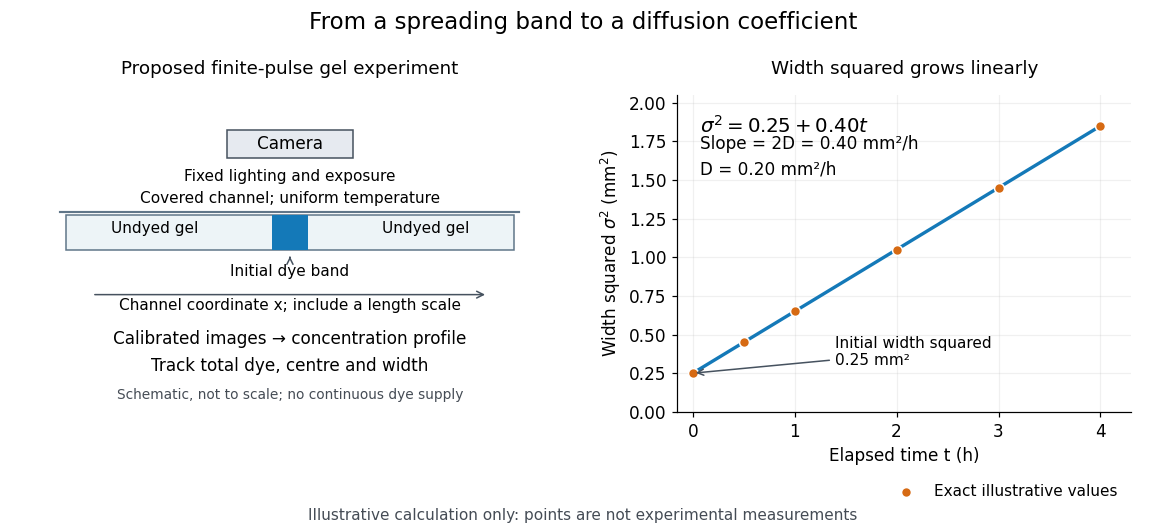
Measuring molecular diffusion from the growth of width squared
. Original schematic of the proposed finite-pulse gel experiment, with an illustrative calculation rather than measured data. A camera records the broadening band. The plotted points are exact samples of with in and in hours; the slope gives the chosen . The schematic is not to scale and is not a reproduction of the published apparatus. Details.For the particularly readable case of an initially Gaussian distribution centred at zero, uniform advection at speed and constant diffusion coefficient give the one-dimensional concentration profileIts centre moves as and its variance grows as . Our illustrative choice and gives widths , and at zero, one and four hours. These are calculated values, not a measured dye coefficient. Once dominates the initial variance, width grows as : four times the elapsed time gives approximately twice the width. A rectangular starting band will not immediately have a Gaussian distribution, although the same width-squared law still applies under the stated assumptions.
Controls and limits of the interpretation. In the proposed experiment, check that stays constant and that the centre remains stationary while the width increases. Include a blank and a uniformly dyed gel photographed over the same period: an apparent signal change there exposes lighting drift, dye fading or evaporation. Repeat with a lower starting dye concentration and a second initial width; agreement of the slopes is a check on constant and on preparation effects. Keep the pulse far from the channel ends and record its faint tails: truncation and background errors can strongly bias a variance. Poor contact, dye binding, chemical reactions or transport in a liquid film can invalidate the simple model. A gel suppresses bulk liquid motion, but its inferred diffusivity need not equal that in the pure solvent. A stationary centre alone does not exclude symmetric flows, and linear width-squared growth alone does not prove a molecular mechanism: turbulence can also produce an effective diffusive description. These are reasons to combine the profile test with the controlled setup.
Rotational diffusion is the random change of a particle's rigid body orientation through Brownian motion. A suspended ellipsoid can turn while its centre hardly moves; translational diffusion instead spreads its position. Random molecular collisions supply fluctuating torques as well as forces. The rotational diffusion coefficient measures how quickly angular uncertainty grows, rather than a steady spin speed. Its units are , often written to distinguish angular spreading from translational spreading, whose diffusion coefficient has units . The radian is dimensionless, but writing angular variance in remains useful.
First identify what the image can reveal. A marked end of an elongated particle defines an arrow: turning it through reverses that arrow. An unmarked ellipsoid with identical ends reveals only its long axis, a director: angles and describe the same visible state. An unmarked perfect sphere has no visible rigid body orientation at all. Tracking its centre cannot measure its rotational diffusion; a surface mark or another identifiable internal direction is needed.
This distinction makes rotational diffusion useful: it measures how long a particle remembers its pointing direction. For an elongated particle, turning also changes which laboratory direction is easiest for translational diffusion. Randomization of rigid body orientation can therefore erase directional preferences in the observed displacement, even though the particle's shape has not changed.
For free planar turning with constant , no imposed torque and negligible inertia, model an unwrapped angle by the stochastic differential equationHere is standard one-dimensional Brownian motion, with increment variance , and brackets denote expected values over repeated realizations. The angular variance is conventionally reported in . “Unwrapped” means recording accumulated turns continuously, rather than resetting the angle at each revolution. Directly subtracting wrapped camera angles creates artificial jumps; for an unmarked ellipsoid the wrapping period is , and resolving successive turns additionally requires sufficiently frequent images.
For a planar arrow , the orientational autocorrelation isFor an unoriented planar axis, use an autocorrelation unchanged by replacing either endpoint angle by that angle plus :The same thus gives arrow and axis correlation times and , respectively, where a correlation time here is the lag at which the relevant curve reaches . A short explanation is enough: has a Gaussian distribution of variance , so its characteristic function gives . The integer selects what the observable can distinguish; it does not change the underlying angular spreading.
For an original numerical example, choose . After , the angular variance is and its root mean square displacement is , although the mean displacement is zero. The planar arrow autocorrelation is , while the planar axis autocorrelation is . Calling both “the orientation correlation” without specifying the observable would hide a factor of four in decay rate.
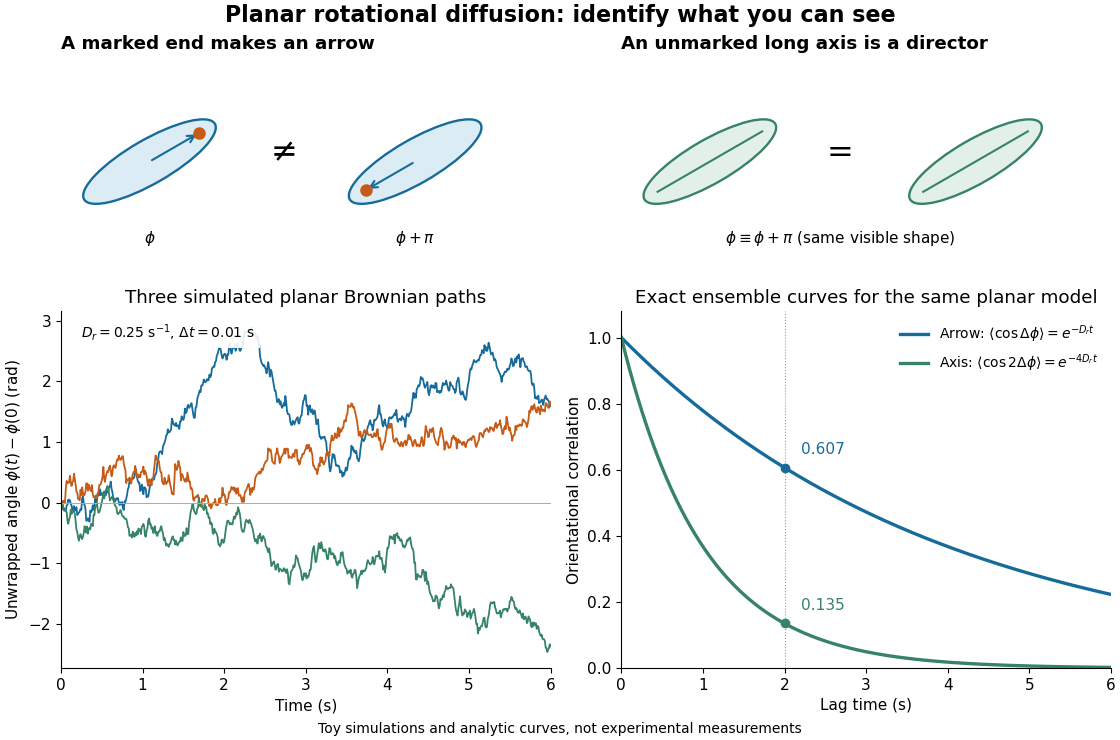
Planar rotational diffusion: arrows, unoriented axes and loss of angular memory
. Original schematics, three simulated Brownian motion angle paths and exact ensemble autocorrelation curves for the chosen . The paths use independent Gaussian distribution increments of variance with . The curves are model predictions, not fits to these three paths or experimental measurements. Both curves concern planar turning; neither is the three-dimensional unit-vector law. Details.For isotropic turning in three dimensions, the tip of a marked unit vector wanders over the unit sphere. Its probability density function obeys the orientational Fokker-Planck equationHere is the Laplace-Beltrami operator on the unit sphere. The factor two follows from the sphere surface derivative identities: , so each mean vector component decays at rate . This is a different orientation space from the circle of planar rotational diffusion, whose corresponding rate is . For the same illustrative and , this three-dimensional autocorrelation is .
One unit vector records a pointing direction, not every aspect of a rigid body's rigid body orientation: rotation about that vector remains unspecified. Also, requires an identifiable arrow. An unmarked ellipsoid's long axis alone does not supply one, and projecting a three-dimensional trajectory onto a camera plane does not automatically produce the planar model.
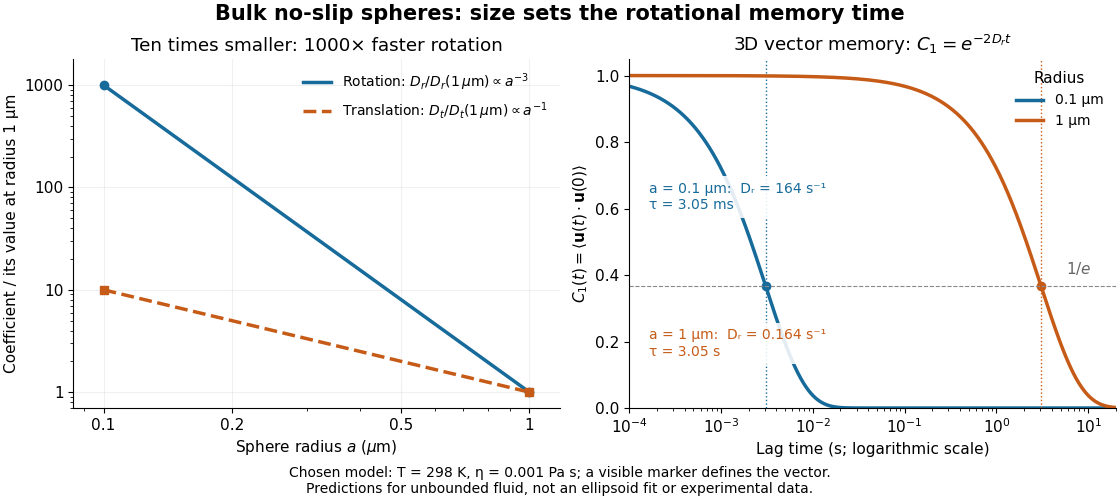
For a sphere of radius in an otherwise stationary, unbounded Newtonian fluid with dynamic viscosity , impose the no-slip boundary condition and the slow-flow assumptions of Stokes flow. The resisting torque on a rotating sphere in Stokes flow is , where is its angular velocity and . Thermal rotational diffusion at absolute temperature then givesHere is the Boltzmann constant; the translational expression is the Stokes–Einstein relation. The ratio has units of inverse length squared, so comparing the numerical values of and without their units is meaningless. At fixed temperature and dynamic viscosity, decreasing radius tenfold increases a thousandfold but only tenfold. This strong size dependence explains why small particles can lose directional memory extremely quickly.
Choose and as illustrative model inputs. Using gives and the following predictions:These are bulk three-dimensional sphere calculations, explicitly not a fit to the confined ellipsoid experiment below. Walls, nonspherical shape and departure from the no-slip boundary condition can change rotational resistance. A visible surface mark is still necessary to read the sphere's turning in an image, even when its rotational diffusion coefficient is well defined physically.
In 2006, Yilong Han and colleagues dispersed plastic ellipsoids in water inside a thin glass cell, using a very dilute suspension to limit particle interactions. A camera on an optical microscope recorded 30 frames per second. Image analysis extracted centre positions and long-axis angles, with reported angular resolution about . Their shape supplied the observable axis. Reflected interference colours calibrated cell thickness; nearly constant particle interference colour checked vertical wandering. One tracked particle had dimensions in an gap. Angular displacement variance grew linearly with lag; displacement resolved along the particle's axes and in the laboratory showed how turning washes out translational anisotropy. These are observations of confined particles: walls alter drag, and slight out-of-plane tumbling affected positional resolution. They do not establish the bulk sphere formula. The paper's Figure 1A–B shows simulations; Figure 1F shows a measured trajectory.[ref]
Brownian Motion of an Ellipsoid by Yilong Han and others. Han et al., Brownian Motion of an Ellipsoid, Science 314 (2006), pp. 626–628; Figures 1D–F and 2A–B: apparatus, angular readout, dilution and height checks, angular variance and translational crossover
For interpreting such images, the director distinction is essential: identical ends give an angle modulo . A continuously unwrapped trace can follow small successive turns, but it does not make the ends physically distinguishable. The invariant planar axis autocorrelation is , and its decay determines through . Separately measuring position and rigid body orientation is what makes the connection between translational anisotropy and loss of angular memory experimentally accessible.
Diffusion of particle position, as distinguished from rotational diffusion of its orientation. Its diffusion coefficient has units of length squared per time.
Articles by others on the same topic

Diffusion is a physical process that describes the movement of particles from an area of higher concentration to an area of lower concentration. This movement occurs due to the random thermal motion of particles and continues until equilibrium is reached, meaning that the concentration of particles is uniform throughout a given space. Diffusion can occur in various states of matter, including gases, liquids, and solids.