Physical optics treats light as a wave, retaining wave amplitude, wave phase and polarization to explain wave interference and diffraction. It predicts how a finite aperture spreads a beam and why overlapping paths can become brighter or darker than either contribution alone.
A pair of illuminated slits makes the distinction from geometrical optics concrete. Ray paths identify the openings and approximate propagation directions, while the relative wave phase determines the fringes on a screen. Reducing optical coherence can wash out those fringes without blocking either path. Physical optics is therefore essential when predicting optical resolution and interferometric signals, even when ray tracing correctly predicts the main image position.
A Bessel-Gaussian beam is a structured optical beam whose Bessel-like transverse oscillations are limited by a Gaussian envelope. For a circularly symmetric zero-order waist-plane model,where is a Bessel function of the first kind, sets the radial oscillation scale and sets the Gaussian envelope. This specifies the initial field; propagating it requires a wave model rather than keeping the same product unchanged at every plane.
An ideal Bessel beam can be constructed from a ring of plane waves with the same longitudinal wavenumber and different transverse directions. Their coherent angular sum gives . The ideal infinitely extended beam has unbounded transverse power. Multiplication by the Gaussian envelope makes the power integral finite, since andFinite transverse extent also means that indefinitely unchanged propagation is no longer guaranteed.
For an original paraxial scale example, let nm, mm and with . The first radial zero of is at , giving . The geometric overlap estimate mm supplies a finite propagation-distance scale, not an exact invariant-range theorem or a measured beam length. The envelope and central-lobe scales answer different questions.
A primary 2023 experiment compared Bessel-Gaussian Gouy phase theory with interferometric measurements. Its apparatus used a 532 nm laser, beam expansion, spatial light modulators, focusing lenses and a camera translated along a rail; Figure 3 documents the interferometer geometry.[ref]
Gouy phase of Bessel-Gaussian beams: theory vs. experiment by Lyubomir Stoyanov and others. Figure 3, p. 13691, apparatus and propagation-plane measurement
Its beam parameters should not be identified with the invented example above.A ringed light intensity image alone does not determine the whole propagated complex field. Measuring wave phase, aperture effects and longitudinal evolution distinguishes a finite structured beam from the mathematical ideal. In particular, the Gouy phase of such a mode should not automatically be replaced by the fundamental Gaussian beam formula.
The angular spectrum representation expresses a monochromatic wave as a superposition of plane waves. In a homogeneous, lossless, source-free half-space with real wavenumber , transverse Fourier transform components propagate independently, providing a useful solution of the Helmholtz equation.[ref]
Use angular frequency and time dependence , and define . Then
The outgoing branch of the angular spectrum has nonnegative real and imaginary parts of for propagation toward . A propagating angular-spectrum component has real ; an evanescent angular-spectrum component has and decays as . The source-plane amplitudes and their complex arguments matter, not just their squared magnitudes.[ref]
The outgoing branch of the angular spectrum has nonnegative real and imaginary parts of for propagation toward . A propagating angular-spectrum component has real ; an evanescent angular-spectrum component has and decays as . The source-plane amplitudes and their complex arguments matter, not just their squared magnitudes.[ref]
Interactive Optics by Sander Konijnenberg, Aurèle J.L. Adam and H. Paul Urbach. Equations374–378, branch convention and evanescent fields
For an original example, a transverse period gives , and . After distance , its amplitude is multiplied by . Such fine spatial detail does not propagate with unchanged amplitude to the far field.
The paraxial angular-spectrum propagator uses . For the source-plane Gaussian beam , its transverse spectrum is proportional to . The on-axis Gaussian integral therefore gives
The denominator produces the axial Gouy phase . This connects the phase shift with interference of transverse spectral components, rather than an abrupt phase jump at the focus.[ref]
The denominator produces the axial Gouy phase . This connects the phase shift with interference of transverse spectral components, rather than an abrupt phase jump at the focus.[ref]
Physical origin of the Gouy phase shift by Simin Feng and Herbert G. Winful. Equations4–12, transverse confinement and Gaussian phase
The scalar propagation formula does not authorize arbitrary independent vector components. A physical electromagnetic field must satisfy the transverse polarization constraint in an angular spectrum; in a uniform source-free medium,. Boundary conditions and source consistency accompany a vector reconstruction.
The transverse polarization constraint in an angular spectrum requires each source-free electromagnetic plane wave component to have electric field orthogonal to its wavevector in the algebraic sense:For an isotropic homogeneous medium with constant permittivity, this follows by inserting a Fourier component into . It restricts the vector fields that can accompany a scalar angular spectrum method calculation.[ref]
Interactive Optics by Sander Konijnenberg, Aurèle J.L. Adam and H. Paul Urbach. Scalar Diffraction Optics, Angular Spectrum Method, vector divergence constraint following the propagation equations
With time dependence and , the relation becomesWhen , the longitudinal field is therefore . It is not an arbitrary third scalar image that can be propagated independently of the first two.
For an original propagating angular-spectrum component with , choosing and forces . Polarization along instead gives a purely transverse-to-axis field for this propagation plane. Thus electromagnetic transversality relative to does not require zero field along the laboratory axis.
For an evanescent angular-spectrum component with , the same choice gives . The dot product is not a Hermitian inner product: there is no complex conjugation of in the Fourier-transformed divergence equation. The imaginary longitudinal amplitude represents a phase relationship, not permission to discard the constraint.
At grazing propagation, , division by fails and the original equation must be used. Boundary conditions, material response and the corresponding magnetic field remain necessary to reconstruct a physical solution. In the strongly paraxial approximation, longitudinal components may be small, but that is an approximation derived from the allowed spectrum rather than a replacement for the vector condition.
The paraxial angular-spectrum propagator is the quadratic-phase approximation to forward free propagation of transverse Fourier transform components concentrated near the optical axis. For real medium wavenumber , write . With time convention , the exact factor is . Expanding at givesafter removing the common carrier .[ref]
The approximation preserves the magnitude of each retained spectral component and changes its wave phase. Recombining those components produces diffraction; it need not preserve the shape or intensity at an individual spatial point. In coordinate space the envelope satisfies the parabolic wave equation, .
Small propagation angle and acceptable accumulated phase error are separate conditions. The first omitted term produces a phase discrepancy of order . For an original component with , the exact difference between approximate and exact phases isIt is about 0.00789 radians at , but about 0.789 radians at . The direction is still only about off axis. Propagation distance matters when phase accuracy is the observable.
For a source-plane Gaussian beam , the spectral width is of order . Thus concentrates the important components in the paraxial region. That provides a reason for the familiar wide-waist condition rather than treating all Gaussian formulas as exact electromagnetic solutions.
A calculation containing substantial evanescent angular-spectrum components or large-angle components requires the exact branch and, when appropriate, the vector transverse polarization constraint in an angular spectrum. The paraxial transfer factor has unit magnitude even at large , so extending it blindly into the evanescent region replaces physical decay by an artificial phase rotation.
The outgoing branch of the angular spectrum selects the longitudinal wavenumber that represents forward radiation and bounded evanescent decay in a specified source-free half-space. For real , time dependence and propagation into ,The first root is positive real and the second positive imaginary. They accompany the factor .[ref]
The scalar Helmholtz equation permits both signs. For , and describe opposite longitudinal phase propagation under the stated time convention. For , the corresponding factors are decaying and growing exponentials. A source-free upper half-space with no incident field from infinity uses the forward, bounded choice.
For an original transverse spatial frequency , the decaying root is . At , amplitude changes by . Choosing the other sign would instead multiply it by approximately 111.3. A sign error can therefore become an enormous near-field propagation error without changing the input data.
This choice is a statement about the physical region and boundary conditions, not an instruction to delete reflected waves from every problem. An interface or cavity can require both propagation directions in a finite region. Likewise, propagation towards negative must use a convention consistent with that region. At , the root is zero and the component is grazing; formulas that divide by need separate attention.
Backward reconstruction of a decayed evanescent angular-spectrum component multiplies measurement error by an increasing exponential. That is an inverse problem's conditioning issue, rather than evidence that the forward outgoing branch should grow. Stating the time convention, physical half-space and radiation condition prevents the square-root symbol from hiding these choices.
An evanescent angular-spectrum component has transverse spatial frequency greater than the medium wavenumber. In a homogeneous lossless medium, with , its forward longitudinal wavenumber is imaginary:It oscillates transversely while decaying away from the source plane. The bounded sign is fixed by the outgoing branch of the angular spectrum.[ref]
For an original transverse period , take , . Then and the amplitude-decay distance is . At , the amplitude is about 0.0658 of its source value, while its squared magnitude is about 0.00433. Amplitude and squared-amplitude attenuation must not be interchanged.
This explains a basic limitation of far-field reconstruction: fine transverse structure can be present at a boundary yet be strongly suppressed before reaching a distant detector. Inverting the factor also amplifies errors. A tiny measured high-frequency component may therefore be an unstable basis for reconstructing fine source detail.
The electromagnetic field is still constrained by Maxwell equations. In particular, remains valid for complex . A single ideal evanescent wave in a lossless medium does not carry time-averaged energy flux normally away from its interface in the same way as a propagating wave. Near-field coupling or a superposition involving another boundary can nevertheless transfer energy, so decay is not a universal prohibition on energy exchange.
An illustrative experiment compares the same patterned source with detectors at increasing distances and accounts for the detector's own spatial response. The decay predicted here concerns a resolved spectral component under the stated homogeneous-medium model, not a guarantee that every observed loss of contrast is evanescence. Absorption, finite aperture and instrument resolution can also suppress structure.
A propagating angular-spectrum component is a transverse Fourier transform component whose longitudinal wavenumber is real in a homogeneous lossless medium. With and the forward outgoing branch of the angular spectrum,Its propagation factor has unit magnitude and a distance-dependent wave phase.[ref]
Interactive Optics by Sander Konijnenberg, Aurèle J.L. Adam and H. Paul Urbach. Scalar Diffraction Optics, Angular Spectrum Method, propagating components and longitudinal wavenumber
For an original component with and , and . It repeats its phase along over distance , even though its wavelength measured along its propagation direction remains . The axial phase period is not an energy-transit time.
Preserving each component's magnitude does not preserve the reconstructed spatial intensity. Different values of accumulate different phases; their coherent superposition changes the interference pattern and can spread a beam. This is the angular-spectrum description of diffraction.
Energy crossing a reference plane also depends on direction. For a vacuum plane electromagnetic wave with electric-field magnitude , the time-averaged Poynting vector has magnitude along the propagation direction. Its normal component through a plane of constant is that magnitude times , where is the vacuum impedance. Equal electric-field magnitudes at angles zero and therefore give normal fluxes in the ratio .
The boundary case is grazing, with and no forward normal phase advance. For , the root becomes imaginary and the component is instead an evanescent angular-spectrum component. These classifications apply to the stated real-wavenumber, lossless model; material absorption requires a consistent complex-wavevector treatment.
Phase-contrast imaging converts spatial phase changes of light into intensity differences by interference with a reference field. In an off-resonant atomic cloud, the optical phase carries information about column density. Weak probing can support repeated measurements with reduced absorption, although destructiveness still depends on detuning and probe strength.
The Huygens-Fresnel principle describes propagation by coherent addition of secondary-wave contributions from a wavefront or aperture. Their complex amplitudes, including relative wave phases, must be summed before calculating light intensity. The Fresnel propagator follows by retaining quadratic propagation wave phase in the paraxial approximation.
Each point on a wavefront acts as a source of secondary wavelets, whose envelope gives the next wavefront. The geometric construction gives refraction from secondary wavelets. The Huygens-Fresnel principle additionally keeps the amplitudes and phases needed to calculate interference and diffraction.
Let a plane incident wavefront first meet a flat interface at , and let another point on that front reach on the interface after . Its path has length . The secondary wavelet from has radius in the second medium; the new wavefront through is tangent to it at . Right triangles with common hypotenuse give and , where both ray angles are measured from the interface normal. Consequently , which is Snell's law. The construction uses phase velocities in homogeneous isotropic media.
Scalar diffraction theory approximates light by one complex field satisfying a scalar wave equation. Aperture propagation is represented by an integral of secondary contributions, with vector polarization of waves and detailed electromagnetic edge conditions suppressed. The approximation is useful for many apertures large compared with wavelength, but is not an exact substitute for Maxwell equations at arbitrary apertures.
In linear scalar diffraction theory, complementary aperture transmissions and give complex fields , where is the unobstructed field under identical illumination. Away from the direct beam in Fraunhofer diffraction, their diffracted fields differ by a sign and have equal intensity. Intensities do not generally add: in particular, complementary on-axis Fresnel diffraction patterns need not have equal intensity. The ideal scalar statement does not incorporate vector boundary details at a real conducting edge.
Spectral phase is the argument of a complex spectral amplitude as a function of frequency. Writing a pulse spectrum as separates its spectral magnitude from the phase function .
Two pulses can have identical spectral intensities and different temporal shapes because their frequency components add with different relative phases. A phase linear in angular frequency shifts the pulse in time; quadratic phase adds group delay dispersion and commonly broadens an initially unchirped pulse. Measuring spectral intensity alone therefore cannot reconstruct the time-dependent electric field; phase-sensitive information is also required.
An interferometer splits or combines coherent wave amplitudes so that an observable depends on their relative wave phase. A Michelson interferometer sends light through two reflected paths before recombination; moving one mirror changes the round-trip optical path difference.
For two detected contributions, under ideal mutual coherence and matched polarization. The varying cross term turns tiny path changes into measurable intensity changes. Stable interpretation requires control of vibrations, beam overlap and optical coherence. A lack of visible fringes can result from those limitations rather than from a lack of light in one path.
A Stern-Gerlach interferometer uses spin-dependent magnetic forces to split matter-wave components and subsequently recombine them coherently. Splitting alone is a spin-position correlation; interference requires restoring sufficient overlap in both position and momentum while controlling the relative phase.
An atom-chip realization uses accurately timed magnetic-field gradients to drive the separating and recombining trajectories. Reading the final spin populations reveals phase-dependent interference after recombination. Residual trajectory mismatch or uncontrolled magnetic noise reduces contrast, explaining why reversing the average force is insufficient by itself to make a complete interferometer.[ref]
Realization of a complete Stern-Gerlach interferometer: Towards a test of quantum gravity by Yair Margalit and others. Abstract and atom-chip full-loop experimental realization
A Rayleigh interferometer compares optical paths through a sample and a reference. A path-length difference shifts the interference phase by . In analytical ultracentrifugation, sample and reference sectors produce concentration-dependent fringe shifts, allowing radial concentration scans without requiring the solute to absorb at the probe wavelength.[ref]
Optical Systems Used for AUC by Beckman Coulter Life Sciences. Rayleigh interference optics: reference sector, refractive-index difference and fringe displacement
In division of wavefront, different spatial portions of an incident wavefront are selected and propagated so that their fields overlap. Double-slit interference is an example. The selected portions need sufficient spatial optical coherence for stable interference fringes.
In division of amplitude, a partially reflecting interface sends parts of the same incident wavefront into separate paths that are later recombined. A Michelson interferometer is an example. The resulting interference visibility depends on relative optical path length, polarization of waves, intensity balance and optical coherence.
An interferogram records detected light intensity produced by interference as a controlled position, phase or delay is varied. In Fourier transform spectroscopy, the variable is the delay between two copies of the same field. Removing the constant background gives a correlation signal whose Fourier transform determines the source's spectral power density, subject to the measured delay window and instrumental response.
An astronomical interferometer combines observations from separated collecting locations to infer angular source structure. Its projected interferometric baseline determines the angular spatial frequency sampled. Amplitude and intensity interferometers measure different coherence observables; a Michelson stellar interferometer combines optical field amplitudes.
A two-element radio interferometer coherently combines signals from two receiving antennas. With equal single-arm wave intensity , projected baseline , free-space wavelength and imposed phase difference , its directional response is the displayed formula. It follows by adding the two complex amplitudes and taking the squared modulus. Near the normal to the baseline, the first null is from a maximum. This narrow response repeats in interference fringes, so a long baseline alone does not give an unambiguous image.
For three collectors whose measured pair phases are , the oriented sum around the triangle cancels the collector-based errors. closure phase retains source phase information, including asymmetry, but does not cancel arbitrary baseline-dependent errors or fill missing spatial-frequency coverage.
The Michelson stellar interferometer, associated with Albert Abraham Michelson, uses separated collectors and beam-redirection optics to produce interference fringes. The collector spacing determines sensitivity to a stellar angular diameter, independently of the final beam spacing at the combiner. The first null for a uniform disk is , where is the full angular diameter. Different surface-brightness laws, including limb darkening, change the null.
Let identical spatially incoherent stellar brightness profiles of equal integrated flux be displaced by projected angles along an interferometer baseline. The Fourier shift property makes their normalized signed coherence . The observed visibility is its absolute value. The slow single-star envelope depends on each star's brightness profile, while the oscillatory factor records projected separation. Unequal flux prevents complete cancellation at the binary minima.
For two identical equally bright stars, zeros of the binary factor occur at , where is separation projected along the baseline. Their repeated spacing is . Multiple samples separate these rapid zeros from zeros of a resolved stellar envelope. Baseline rotation is needed to recover an unknown two-dimensional separation direction; the first zero alone does not determine both diameter and separation.
Two identical uniform circular discs of angular diameter and equal flux have , , with limiting value one at . Multiplication by gives their signed binary coherence. Its first single-disc envelope zero is , while the binary modulation has a separate scale . Limb darkening and other nonuniform profiles change the envelope, not the elementary Fourier shift factor.
Fresnel diffraction describes diffraction when the quadratic propagation wave phase across an aperture must be retained. Its Fresnel propagator becomes the Fraunhofer diffraction description when that curvature is negligible.
A Fresnel diffraction pattern is a map of how propagation changes the wave interference of light from an aperture. It can resemble the opening, develop bright and dark structure near its edges, and eventually approach a Fraunhofer diffraction pattern. The controlling comparison involves wavelength, opening size and propagation distance together; a distance large compared with the opening need not give the far field.
For a monochromatic wave, use time dependence , wavenumber and complex amplitude . Let be the transmitted field immediately behind an aperture in the plane . In a homogeneous medium, the scalar paraxial approximation givesThis is the two-transverse-coordinate Fresnel propagator, with its carrier restored. It adds complex amplitudes before taking their squared complex modulus to obtain light intensity. It is a scalar paraxial approximation, rather than a full vector solution of Maxwell equations.[ref]
Scalar Diffraction Optics. Interactive Optics by Sander Konijnenberg, Aurèle J.L. Adam and H. Paul Urbach; Fresnel Approximation, equations (381)–(385), and the following paraxial-wave-equation remark
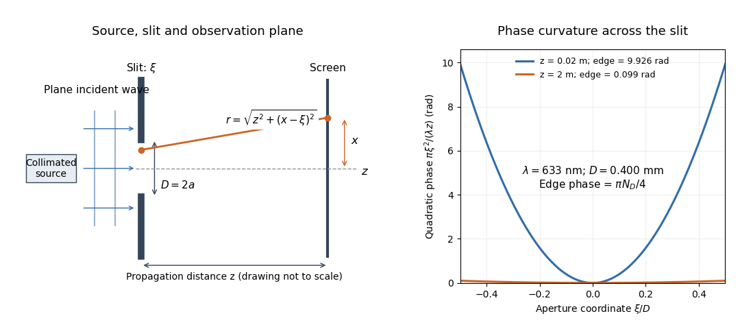
The source in this constructed geometry supplies a plane wave; the observation screen is a plane perpendicular to the optical axis. The right panel isolates the aperture-dependent wave phase that distinguishes Fresnel diffraction from Fraunhofer diffraction. Its vertical scale is in radians, and the drawing's lengths are schematic.
Keeping this wave phase is useful when transporting a field between nearby optical components: both the shape and the complex amplitude matter for subsequent wave interference. A particularly striking feature is that propagation can create a dark centre even from a uniformly illuminated symmetric aperture; the incident wave amplitudes need not be unequal for their outgoing contributions to cancel.
For normalized Fresnel integrals , an interval aperture contributes the chord between its two limiting points on the Cornu spiral. The full unobstructed field is , so its squared magnitude is2. Comparing to only the half-plane limit instead of this full chord introduces a factor-of-four normalization error. The formula compares power at one observation point under the same illumination and propagation factors.
The largest radius of the normalized Cornu spiral occurs on its first outer turn at , where . Oddness makes the chord from to attain twice that radius, while the triangle inequality bounds every other chord by the same length. The interval is therefore the strongest freely selectable connected aperture at that observation point, with normalized point power about1.80142. Signed physical limits follow from . Existing openings can constrain this optimization.
A Fresnel diffraction aperture can increase the detected intensity at one selected observation point by removing contributions that would otherwise interfere destructively there. The increased local signal is a redistribution of transmitted radiant power, not an increase in total energy supplied by the incident beam.
For a passive absorbing screen under fixed illumination, closing part of an aperture cannot increase the total transmitted radiant power. Nevertheless the remaining complex amplitudes can have a larger sum at a particular point. Comparing the single-point response with a measurement integrated over the whole transmitted field distinguishes the largest contiguous Fresnel aperture optimization objective from an efficiency claim.
If a screen already has an interval hole, additional removal cannot reduce that hole. A connected final aperture must contain it, imposing lower/upper endpoint constraints on its Cornu spiral chord. The unrestricted longest chord need not be feasible. For an existing interval , constrained chord maximization gives approximately , , with point-power ratio1.60257. The two aperture endpoints, rather than just a nominal Fresnel-zone width, determine the received field.
For an opaque half-plane whose edge lies height above the direct source–receiver ray, the paraxial parameter is . The unobstructed half-aperture supplies the Cornu spiral chord from to infinity. Division by the full-aperture chord gives the displayed intensity transmission. It is at grazing incidence, approaches one well into the illuminated region and tends to zero deep in shadow.[ref]
A diffraction-loss ratio is normalized to the unobstructed intensity at the same receiver position. With a point source that unobstructed intensity changes as inverse source–receiver distance squared. Moving the receiver can therefore decrease the transmission ratio while increasing its absolute received intensity. The two curves require separate normalization; a Cornu-chord plot alone omits geometric spreading.
A scalar aperture approximation that sums the secondary waves reaching an observation point. For a point source with incident spherical amplitude , one common forward-normal convention isHere and are source-to-aperture and aperture-to-observer distances and is an obliquity factor. The Fresnel diffraction approximation retains quadratic path phase; Fraunhofer diffraction additionally neglects the quadratic phase across the aperture. Kirchhoff boundary assumptions do not give an exact electromagnetic solution at a sharp edge.
A concentric diffractive focusing element with successive zone boundaries chosen to differ by half a wavelength of optical path to a focus. Alternating transmitting and absorbing zones suppress cancellation between neighboring half-period zones. For an incident plane wave, the paraxial boundaries satisfy . The outermost zone width controls the finest transverse scale, and the focal length varies with wavelength.
For a plane wave incident on a flat zone plate, the path difference from radius to axial focal distance is . Setting it equal to gives the title relation. The paraxial limit is , and the fine outer-zone width is approximately . Alternately removing half-period annuli makes the remaining contributions reinforce at the principal focus. Choosing the number of zones sets the aperture and fabrication scale, not the principal focal distance independently of these radii.
For uniform coherent plane-wave illumination, an ideal binary amplitude zone plate transmits alternate Fresnel half-period zones. If complete odd zones are open, every one contributes approximately twice the unobstructed axial complex amplitude, in the same phase, and . This is a local light intensity gain relative to removing the plate and outer stop. It differs from comparison with a finite clear aperture: an aperture containing an odd integer number of half-period zones has axial intensity , giving plate-to-aperture ratio . Neither gain is a total power efficiency.
At the geometric shadow boundary of a straight opaque half-plane, the transmitted Fresnel integral is exactly half the unobstructed complex amplitude for ideal point illumination. The Cornu spiral chord is from its origin to one limiting endpoint, rather than between both limiting endpoints. Therefore and . Half the unobstructed intensity would confuse a field fraction with its square. Edge thickness, source extent and alignment can modify the ideal result.
The Arago spot is the bright axial point in the shadow of a circular obstruction under suitably coherent illumination. In ideal scalar diffraction theory, secondary fields from the circular edge arrive in phase on axis. Fresnel diffraction by an opaque disk gives an axial intensity equal to the unobstructed intensity in its paraxial model; this is not a claim that the whole geometric shadow is bright.
Under the same scalar paraxial assumptions as Fresnel diffraction by a circular aperture, Babinet's principle gives the complementary opaque-disk field on axis. Its axial intensity equals the unobstructed intensity, producing the Arago spot inside the geometric shadow. The off-axis pattern depends on the full Fresnel integral; it is not obtained by subtracting aperture intensities from the incident intensity. Finite source size, misalignment and imperfect circular edges reduce the ideal spot contrast.
For a circular aperture of radius , paraxial plane-wave illumination and propagation distance , define . On axis, the radial Fresnel diffraction integral normalized by the unobstructed field givesFor a finite axial point source a distance before the aperture and detector a distance after it, replace by in the phase. The formula assumes illumination amplitudes and obliquity factors approximately constant across the aperture. Odd and even numbers of Fresnel half-period zones give bright and dark axial extrema; large local intensity is compatible with global conservation of energy.
A Fresnel half-period zone is a region of an aperture whose optical path to an observation point differs from the axial path by an interval of half a wavelength. For an axial optical point source a distance before the aperture and an axial observer a distance beyond it, the paraxial path excess at aperture radius is . The outer radius of zone is thereforeSuccessive zones contribute approximately opposite phases to the Huygens-Fresnel principle integral. The finite source distance matters: using the plane-wave formula requires .
For an axial point source a distance before a square aperture and an observer a distance beyond it, source and observation wave phase curvatures add: . With aperture side , put . Separation into two one-dimensional Fresnel integrals gives the field normalized to its unobscured value,At an off-axis observer , centre the dimensionless coordinates on and . If are the directed Cornu spiral chords between the corresponding aperture-edge parameters, . This is a product of complex interval factors, rather than a sum of two intensities. The unobscured field is evaluated at the same observation point and includes its common propagation wave phase.
The quadratic wave phase follows from an ordinary distance calculation. Write . The Taylor expansion of the distance to a screen point isIn the slowly varying propagation prefactor, suffices. In the complex exponential , however, a small distance error is multiplied by the large wavenumber . Retaining the quadratic term while dropping the quartic term requires both and over the contributing aperture and the screen region being considered. The second condition is a wave phase accuracy requirement; the first is the geometric paraxial approximation.
Expanding the retained quadratic term separates three effects:The outside quadratic factor changes the wave phase at each screen point but has unit complex modulus, so it leaves that screen's light intensity unchanged. The quadratic factor inside the integral changes relative wave phases between contributions from different aperture points, so it changes their wave interference. The remaining linear factor supplies a Fourier transform. Fraunhofer diffraction drops the aperture quadratic factor when it is nearly constant; it does not require dropping the screen quadratic factor when predicting a later coherent field.
There is also a useful proof from the Helmholtz equation. Substituting gives . Neglecting yields the parabolic wave equation. A transverse Fourier transform evolves each spatial frequency by , using the transform kernel . Its inverse Fourier transform is the quadratic Fresnel propagator kernel above. Thus quadratic wave phase in space and quadratic wave phase in spatial frequency are two views of the same propagation.
A Fresnel number compares squared aperture size with the product of wavelength and propagation distance. For an optical slit of full width , explicitly distinguish the full-width and half-width conventions:The full-width convention is used throughout the Fresnel slit propagation example below. The definition also appears in the Delft treatment.[ref]
Scalar Diffraction Optics. Interactive Optics by Sander Konijnenberg, Aurèle J.L. Adam and H. Paul Urbach; Fresnel and Fraunhofer Approximations, equations (390)–(392): aperture diameter convention
For uniform incident wave phase, makes the omitted aperture wave phase small and gives the Fraunhofer diffraction regime. When is of order one or larger, retain it and use Fresnel diffraction, provided the paraxial approximation still holds. These are continuous changes in accuracy, rather than a physical boundary at one selected number. For a rectangular aperture, check both transverse dimensions. Incident wavefront curvature contributes its own wave phase through ; the aperture-to-screen Fresnel number alone does not describe a spherical source's illumination.
The scaling is revealing: doubling the optical slit width at fixed wavelength and distance multiplies the Fresnel number by four. Maintaining the same Fresnel number then requires four times the distance. Two systems can consequently have the same dimensionless pattern despite very different physical lengths.
Consider a uniform plane wave of unit complex amplitude transmitted by an ideal optical slit of full width . Treat the field as invariant along the optical slit height: this is one-dimensional transverse Fresnel propagation, so the prefactor is , rather than the two-dimensional prefactor . Removing the carrier givesHere is incident irradiance. This infinitely long slit model describes a transverse cut away from the ends of a sufficiently long physical slit; its finite conserved quantity is transmitted power per unit optical slit height.
Put and . Substitution reduces the integral toThis form separates the pattern's shape from its physical scale. Reflection proves , so the light intensity is an even function of . At , direct integration gives , with limit one at . Hence the Fraunhofer diffraction comparison is the squared sinc function. In this paragraph the unnormalized sinc function takes argument .
For an original example, choose wavelength and full width . At , , and the edge-to-centre wave phase change is radians. At , , and that wave phase change is only radians. Even the nearer screen is fifty slit widths away; that geometric comparison alone misses its strong Fresnel diffraction.
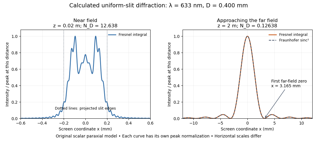
Original calculated Fresnel diffraction profiles of a 0.400 mm slit at 633 nm, compared with the Fraunhofer diffraction shape
. Details. These are numerical predictions from the displayed scalar integral, using the composite trapezoidal rule, rather than measured profiles. Each curve is divided by its own peak light intensity; the two horizontal scales differ. At 2 cm the computed central irradiance is about , with brighter off-axis maxima. At 2 m it is about and is the peak. The dashed Fraunhofer diffraction curve has its own central normalization; its first zeros are at . The finite-distance Fresnel diffraction curve remains slightly nonzero there.
Normalization hides the brightness change, but not the change in shape. The Fourier transform propagation multiplier has unit complex modulus, so Plancherel theorem givesThis is conservation of transmitted power per unit height in the ideal scalar model. An integral over only the displayed screen interval misses the tails; a peak-normalized profile is not a unit-integral probability density. Spreading and decreasing brightness together preserve the transmitted power.
A documented experiment uses curved illumination rather than the uniform Fresnel slit propagation model. Laboratory Exercise No. 4: Diffraction, MIT 6.237, Fall 2024, printed pp. 5–6, gives a helium–neon laser at , a microscope objective optical lens, a circular aperture and a screen 5–40 cm from the object. Preparation includes comparing central brightness in Fresnel diffraction and Fraunhofer diffraction. A 40× objective produces a nonplanar incident wavefront; the opening is placed less than 1 cm from it. With objective-to-screen distance fixed, students move the opening, sketch patterns, and record positions of consecutive central nulls to estimate aperture size. The Fraunhofer diffraction pattern supplies a regime comparison. A separate spherical-obstacle task observes a bright centre inside the shadow. The handout supplies procedures, rather than measured distances or profiles.[ref]
The circular-opening test probes cancellation of complex amplitudes at the centre while the source wavefront curvature changes. To interpret it, include that curvature in the aperture field and use a circular aperture, rather than substituting the plane-illuminated Fresnel slit propagation profile. Useful additional controls are to retain the same laser and opening, centre the illumination, repeat position readings and check background with the beam blocked. If a camera replaces the visual screen readout, avoid saturation and calibrate its position scale. Alignment, imperfect aperture edges, illumination variation and limited contrast near a null constrain the inferred size. A bright central obstacle spot illustrates why the sharp shadows of geometrical optics can fail; it does not imply that every Fresnel diffraction pattern has a bright centre.
A fundamental Gaussian beam is an ideal beam of light whose transverse wave amplitude has a Gaussian function profile. Here consider a circularly symmetric beam in vacuum, with propagation along , two transverse coordinates , and radius from the optical axis. With the beam waist at , total power , and vacuum wavelength , its time-averaged light intensity, meaning irradiance in , isHere is the minimum beam radius, and is the Rayleigh range. Far from the beam waist, with beam divergence half-angle . These are the fundamental circular Gaussian beam laws within the scalar paraxial approximation, appropriate when and the beam divergence is small. The underlying envelope solves the parabolic wave equation exactly; this does not make it an exact vector solution of Maxwell equations. [ref].
The radius convention matters. Writing for the complex wave amplitude envelope, the same is the wave amplitude radius and the light intensity radius:At these ratios are and , respectively. The light intensity radius is instead . None of these radii is a sharp edge: the ideal Gaussian function has nonzero tails at every finite radius. Kogelnik and Li explicitly use the wave amplitude radius in their fundamental-mode treatment. [ref]
https://dielslab.unm.edu/sites/default/files/Kogelnik66_0.pdf. Herwig Kogelnik and Tingye Li, Laser Beams and Resonators, Applied Optics 5, 1550–1567, 1966, §3.2
.For a numerical example, take vacuum wavelength and beam waist radius . Substitution gives Rayleigh range and far-field beam divergence half-angle . At , the beam radius is and the on-axis irradiance is half its waist value. At the same wavelength, halving the beam waist radius to quarters the Rayleigh range to and doubles the beam divergence half-angle to . At fixed power, that smaller beam waist also quadruples the peak irradiance.
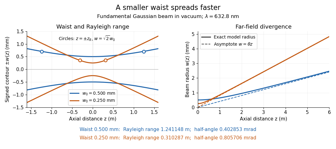
Gaussian beam radii at 632.8 nm: a smaller beam waist gives a shorter Rayleigh range and greater beam divergence
. Details. The contours in the left panel are in a plane through the optical axis; they mark an light intensity level, not an outer boundary. The right panel compares the exact model radii with the far-field asymptotes . The horizontal and vertical axes use different length units, so the drawn slopes are not physical angles.
The normalization expresses conserved power during free propagation. In transverse polar coordinates, an annulus has area , soA proof outline is the substitution in this integral. Spreading reduces peak irradiance as while increasing transverse area as , leaving power unchanged. In particular, the disk of radius contains , or , of the total power; the local light intensity at its rim is only of the on-axis light intensity. These are different quantities.
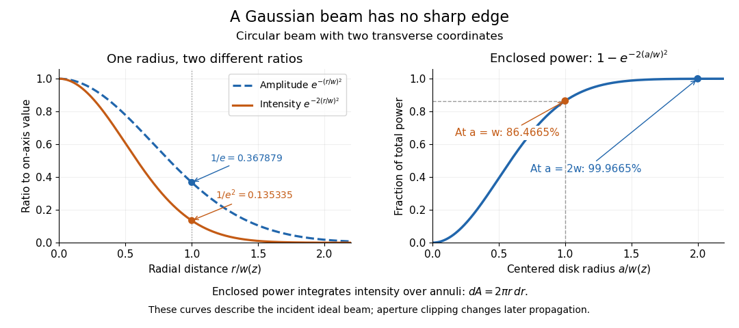
The left panel compares normalized wave amplitude magnitude and irradiance; the right panel integrates the transverse area to show enclosed power. For an ideal absorbing circular aperture of radius centered on the optical axis, the same fraction gives the power passing the aperture at that plane. An aperture of radius clips about of the incident power; radius clips only , or . After clipping, extra diffraction means the transmitted field no longer obeys the unmodified ideal Gaussian beam law. Every finite aperture cuts some ideal tail. Kogelnik and Li distinguish their large-aperture beam analysis from their finite-aperture diffraction analysis. [ref]
https://dielslab.unm.edu/sites/default/files/Kogelnik66_0.pdf. Kogelnik and Li, 1966, §§3–4
.The useful tradeoff is that a small bright spot cannot remain narrow indefinitely. An optical lens can create a smaller beam waist, but diffraction then makes the beam spread faster. The particularly simple relation ties localization directly to beam divergence. A proof outline for the propagation law starts with . The parabolic wave equation separates into two transverse factors, and a Gaussian integral in each coordinate givesHere is dimensionless and is the wavenumber; the carrier convention is , with angular frequency . Taking the squared complex modulus gives the stated and its light intensity scaling. Each transverse factor contributes , explaining the prefactor here and the different prefactor in the preserved Gaussian beam with one transverse coordinate.
Historically, Gaussian beam theory developed alongside early laser resonator theory and lens-guided transmission. In their 1966 review, Kogelnik and Li credit Boyd and Gordon, and Goubau and Schwering, with early beam treatments; they summarize earlier work rather than claim the whole construction as a new discovery. Their paper brings beam propagation, focusing and finite-aperture diffraction into a common practical account. [ref]
https://dielslab.unm.edu/sites/default/files/Kogelnik66_0.pdf. Kogelnik and Li, 1966, introduction and §3
.Fourier localization of a Gaussian beam expresses the tradeoff between a narrow transverse field and a broad distribution of transverse spatial frequencies. At a waist, takeTwo Gaussian integrals giveReducing therefore broadens the angular spectrum method representation rather than merely shrinking a picture in the same set of propagation directions.[ref]
Physical origin of the Gouy phase shift by Simin Feng and Herbert G. Winful. Equations 4–12, transverse confinement, spectral description and Gaussian phase
Widths must state their weighting. Normalize and to define transverse position and transverse-wavenumber distributions. Their one-coordinate standard deviations areThese are optical field-width statements under the stated Fourier convention, not an inference that each ray has simultaneously measured position and angle. Using amplitude widths instead would give different numerical factors.
For a strongly paraxial spectrum, and . The usual far-field Gaussian light intensity half-angle is . For original nm and mm, mm and mrad; the conventional divergence half-angle is about 0.4029 mrad. Halving the waist doubles both angular measures.
An illustrative apparatus places a camera in a plane conjugate to the waist and another measurement at a lens's back focal plane, where transverse spatial frequency maps to position in the paraxial model. Comparing widths tests localization and angular spread, provided magnification, focal length and detector response are accounted for. Finite aperture clipping changes the field and produces extra spectral structure, so the exact Gaussian width product cannot simply be assigned to every clipped beam.
The same spectrum also bounds the paraxial approximation: keeps most amplitude at transverse wavenumbers much smaller than . Strong focusing can require vector polarization constraints and a nonparaxial propagation model.
The Gouy phase describes the additional axial phase associated with a focused wave relative to a plane wave. For a fundamental circular Gaussian beam with beam waist at and Rayleigh range , defineWith the carrier convention , the on-axis field phase is up to a constant. Thus the signed additional phase is in this convention; defining the positive function does not reverse the physical prediction.[ref]
Physical origin of the Gouy phase shift by Simin Feng and Herbert G. Winful. Equation12, printed p.486, sign convention for the Gaussian phase contribution
The complex field prefactor gives a short derivation. The normalized Gaussian propagation factor isIts modulus describes the on-axis amplitude reduction; its argument is the additional phase. An intensity measurement alone loses this argument, so measuring the beam's width and brightness does not directly measure the Gouy phase.
As runs from far before to far after the waist, runs continuously from to . The total additional phase change has magnitude , but is not a discontinuous jump at the waist. For stipulated and , . Between and , the additional phase changes by ; the far-field-to-far-field limit gives .
The number of confined transverse directions matters. A Gaussian beam with one transverse coordinate has prefactor and half this phase contribution. Simin Feng and Herbert G. Winful's primary analysis relates the effect to transverse confinement and the angular spectrum representation: a localized beam includes transverse wave-vector components, affecting axial propagation.[ref]
Physical origin of the Gouy phase shift by Simin Feng and Herbert G. Winful. Equations4–12 and line-focus versus point-focus discussion, pp.485–486
An illustrative Gouy phase interferometry experiment overlaps the focused beam with a coherent reference beam and records the interference phase at different axial planes. Removing the ordinary optical-path contribution and accounting for wavefront curvature isolates the axial phase change. This is a proposed measurement outline, not an experimental result reported by the cited theoretical paper. In an optical cavity, related phase contributions help determine the resonance condition and distinguish transverse modes.
Gouy phase interferometry compares a focused field with a coherent reference to recover the additional Gouy phase. Beam brightness alone discards the phase. An interferometer converts a relative field phase into intensity modulation, but the optical paths and reference wavefront curvature must be modeled.
A published 2023 experiment by Lyubomir Stoyanov and colleagues used a Mach-Zehnder interferometer to study Bessel-Gaussian beams. Its setup included a 532-nanometre laser, beam expansion, two spatial light modulators, focusing lenses and a CCD camera on a rail to follow propagation after the focus. Its Figure 3 also describes a single-lens interferometer arrangement for stronger focusing.[ref]
Gouy phase of Bessel-Gaussian beams: theory vs. experiment by Lyubomir Stoyanov and others. Figure 3, printed p. 13691, apparatus caption
Structured modes need their own phase model; that experiment should not be silently interpreted as a fundamental-Gaussian measurement.A separate original protocol illustrates four-step phase retrieval. At one detector point, apply controlled signal-arm phases while the beam intensities remain fixed. Write
This phase-shifting interferometry formula removes the unknown common intensity background and positive modulation amplitude . It returns phase modulo ; phase unwrapping requires continuity information between sampled positions. If the interference visibility vanishes, the phase is not observable by this formula.
This phase-shifting interferometry formula removes the unknown common intensity background and positive modulation amplitude . It returns phase modulo ; phase unwrapping requires continuity information between sampled positions. If the interference visibility vanishes, the phase is not observable by this formula.
For a synthetic coherent Gaussian/reference pair, use reference intensity 1 and signal intensity , with . Then , and after common path phases are removed. At , the four intensities are , giving . At , the first intensity is still , but the quadratures reverse and the retrieved phase is .
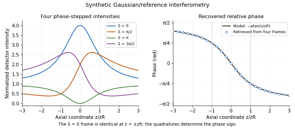
Original synthetic four-step interferometry of a Gaussian beam: symmetric single-frame readings become distinguishable through phase quadratures. No experimental data are shown.
Details. Curvature bias in Gouy-phase measurements is important away from the axis: the signal adds to its spatial phase. Fit or remove that term when using multiple pixels, retain calibrated phase steps and account for drift between frames. The recovered phase combines all coherent optical-path contributions until those controls isolate the Gouy phase.
Curvature bias in Gouy-phase measurements occurs when a spatially varying wavefront-curvature wave phase is mistaken for the axial Gouy phase in an interferometric comparison. For a fundamental Gaussian beam with time convention , the signal wave phase containsA curved reference contributes its own quadratic wave phase. After subtracting common axial path terms, the measured relative wave phase isThus a phase-retrieval algorithm can work exactly while the subsequent physical interpretation is biased. The Gaussian confinement wave phase and its arctangent dependence are derived in the primary theoretical treatment.[ref]
Physical origin of the Gouy phase shift by Simin Feng and Herbert G. Winful. Equations 4–12, Gaussian field phase and confinement
For an original example with a planar reference and stable path wave phase, let and . At and fixed detector radius , the curvature term is 0.5 radians. The true axial contribution is , whereas that off-axis pixel gives radians. At the curvature term reverses. Comparing those two axial planes at this fixed radius gives a wave phase change , differing from the axial Gouy change by one radian.
The effect is observable even where the signal is appreciable: at , is inside the plane's Gaussian radius . Avoiding only dim pixels does not remove curvature bias.
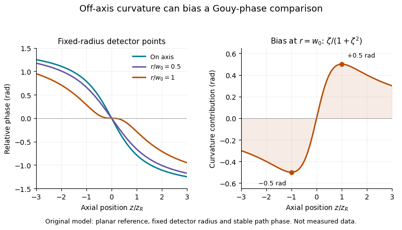
A useful measurement fits the spatial quadratic wave phase, identifies the beam center and reference curvature, and extrapolates the relative wave phase to the axis. Tilt, decentering and path drift require their own terms; averaging several pixel phases is not automatically equivalent to measuring the on-axis wave phase. Phase unwrapping can be required before fitting a wave phase profile.
The primary 2023 Bessel-Gaussian experiment documents focusing optics and a rail-mounted camera in its interferometer.[ref]
Gouy phase of Bessel-Gaussian beams: theory vs. experiment by Lyubomir Stoyanov and others. Figure 3, p. 13691
It motivates tracking both propagation position and wavefront geometry, but its structured-mode observations must not be silently reclassified as measurements of the illustrative fundamental-Gaussian model above.For a circular Gaussian beam with intensity proportional to , the displayed is the intensity radius. Its minimum is the beam waist radius, while the larger radius at a cavity mirror is not itself a waist. The Rayleigh range is .
The complex beam parameter combines a Gaussian beam's wavefront curvature and spot radius : . With , the beam waist is . A real paraxial ray transfer matrix maps it by . Positive imaginary part selects the physical finite-width branch in this convention.
A real paraxial ray matrix transforms a Gaussian beam parameter by the displayed fractional-linear map. For a lossless round trip with determinant one, a fixed point with positive imaginary part generically requires . Scalar matrices are degenerate exceptions: their fractional-linear map fixes every physical beam parameter even at the boundary. Finite apertures and resonance phases impose additional physical constraints.
The beam waist is the narrowest cross-section of a freely propagating Gaussian beam. Its radius uses the wave amplitude , or light intensity , convention; its diameter is . Specifying a “spot size” without saying radius or diameter can introduce a factor-of-two error. Within the scalar paraxial approximation, the wavefront at the beam waist is planar. The minimum radius sets both the Rayleigh range and the far-field beam divergence.
The Rayleigh range of a fundamental Gaussian beam in vacuum is the positive axial distance from the beam waist at which its radius grows from to . Thus its contour area doubles and its peak irradiance halves. Within , the radius stays at most ; for , beam divergence dominates. At fixed vacuum wavelength, the Rayleigh range scales quadratically with the beam waist radius. The formula here uses the vacuum wavelength, not an unlabelled wavelength in a material.
For the free parabolic wave equation , input with propagates asThe branch is continuous from . One-dimensional transverse Fresnel propagation or two Gaussian integrals prove the formula. With , the squared envelope is . The amplitude power is because there is only one transverse coordinate. A two-transverse-coordinate Gaussian beam instead has power when both coordinates share the same .
Beam divergence describes the angular spread of a beam away from its optical axis; specify the radius convention and whether the quoted angle is a half-angle or full angle. For the fundamental Gaussian beam in vacuum, the far-field light intensity radius obeysHere is the small-angle half-angle in radians under the paraxial approximation; the full angle is . The geometric asymptote has angle , approximated by in this regime. Other beam profiles need their own beam divergence definitions and propagation laws.
Phase conjugation creates a returning monochromatic wave whose spatial complex amplitude is proportional to the complex conjugate of the incident field. Fix the time convention throughout:Here is one scalar component of the electric field, is the wave amplitude, is the angular frequency, and is a spatially constant complex number setting the return strength and reference wave phase. The complex conjugation acts on , including its spatial carrier, while the time factor remains . Conjugating both factors would merely give another representation of the same real field. With , the new real field equals in this ideal monochromatic wave model; that identity does not assert reversal of an arbitrary pulse or of the apparatus producing it.
The spatial wave phase becomes , so the local wavevector changes from to . For example, with becomes : both components of the wavevector reverse. In a transparent stationary medium with isotropy and positive refractive index, light rays follow the wavevector, giving counterpropagation. The same wavefronts now have opposite propagation normals. This is why phase conjugation can return a distorted beam toward its origin: it reverses the detailed spatial wave phase, rather than requiring that wave phase to be flat.
The attractive application is correction of optical aberrations accumulated on an outward trip. The return uses the distortion itself as the prescription for correction, as the original thin phase-plate cancellation by phase conjugation example makes explicit. An experimentally accessible implementation measures the spatial wave phase and uses a spatial light modulator to generate its negative; digital optical phase conjugation describes an inspected 2010 demonstration of recovery through multiple scattering.
A phase-conjugate mirror is an optical device that implements phase conjugation at its return surface. It may generate the return using an independently supplied beam, as in digital optical phase conjugation; its name specifies the field transformation, rather than a particular reflecting material. Conjugating the transverse complex amplitude and launching the returning longitudinal carrier produces the complete reversed wavevector. A spatially constant leaves the shape of the wavefront unchanged; a spatially varying would add its own wavefront error.
An ordinary flat mirror obeys the law of reflection. At a surface , its reflected plane wave has wavevector , whereas a phase-conjugate mirror returns . Ordinary specular reflection preserves the tangential wavevector. At normal incidence a single plane wave can therefore look identical in the two cases, apart from an overall wave phase and strength; oblique incidence or a curved wavefront reveals the distinction. In boundary-envelope notation an ideal ordinary mirror multiplies the incident complex amplitude by a constant reflection factor , while an ideal phase-conjugate mirror returns its complex conjugate times .
Consider an optical point source at , a uniform transparent medium, and a flat return surface . A light ray with slope reaches . A phase-conjugate mirror reverses its full direction and returns it to . An ordinary mirror reverses only its normal direction; its returning light ray reaches at . Thus rays with at return to with ordinary specular reflection, but all return to under ideal phase conjugation. These are stipulated geometric coordinates, not laboratory measurements.
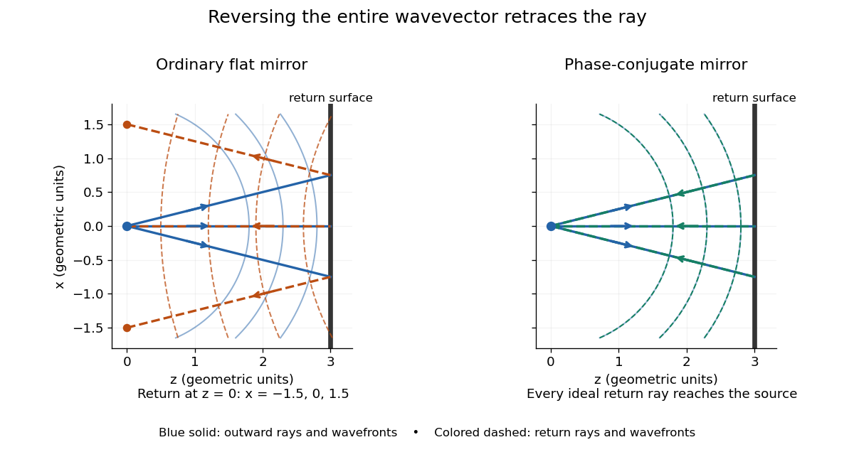
Solid blue curves mark outward wavefronts; dashed curves mark returning wavefronts. In the phase-conjugate mirror panel the returning curves coincide with the outward ones, and the arrows reverse on the same light rays. The diagram uses equal spatial scales. In geometrical optics, reversing each light ray in an unchanged medium with wave reciprocity retraces its route. At the optical point source itself, the ray construction becomes singular and diffraction sets the physical focal size.
A wave-level proof outline applies to a stationary scalar medium with real refractive index and no wave absorption. Writing for the vacuum speed of light, its Helmholtz equation isAll coefficients are real, so complex conjugation gives the same Helmholtz equation for . The conjugated outgoing boundary data select the incoming solution. This explains the connection between phase conjugation and retracing, provided the required incoming field is supplied over the necessary aperture. It also exposes the limits: wave reciprocity alone does not imply absence of wave absorption; conjugation of complex material coefficients would describe a different medium. Loss, an incomplete aperture, a changing medium or failure of wave reciprocity can prevent exact reconstruction. Intensity-dependent material changes need a separate analysis and are not covered by this linear proof.
Model a thin transparent plate by a lossless reciprocal phase screen with transmission at the chosen angular frequency. Both passages multiply the local field by the same : reversing travel does not by itself change the sign of an accumulated optical path length. Assume the plate is stationary, the two passages use corresponding transverse positions, and the plate is adjacent to the return surface or perfectly reimaged onto it. Ignore propagation between these reference surfaces, wave absorption, clipping and intensity-dependent changes. Take the incident boundary envelope to be . Outward transmission gives . Ideal phase conjugation and the second transmission then giveThis is a complete short proof of cancellation in the specified phase screen model. For an ideal ordinary mirror with constant reflection factor , the corresponding envelope is : the extra wave phase is , rather than zero. A constant reflection wave phase changes neither conclusion.
For an original toy optical aberration, let on , take , and chooseThe even term adds symmetric curvature and the odd term makes the two sides unequal. The outward wave phase is ; immediately after ideal phase conjugation it is ; after the second passage it is zero. At , the outward values are , while an ordinary mirror's completed return has values . All wave phases here are unwrapped relative to the central ray and are otherwise equivalent modulo . At a stipulated vacuum wavelength , these outward errors correspond to optical path length errors of . These are chosen values; they are not observations or physical plate thicknesses.
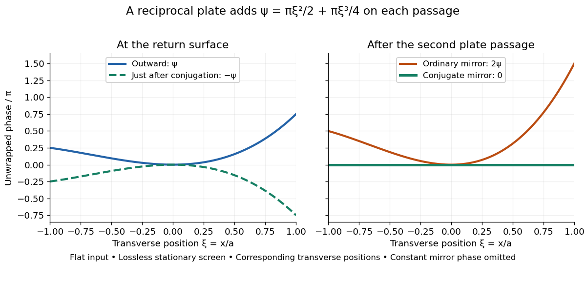
Original thin phase screen example: sign reversal at conjugation and cancellation after the second passage
. Details. The wave phase plots make a subtle distinction visible: the field is still curved immediately after phase conjugation, and becomes flat only after crossing the same plate again. More generally, conjugation restores , not a universally flat wavefront. If the plate instead has transmission with real , the return is . Its plate-induced wave phase cancels but its lost wave amplitude does not recover. If the return plate has changed to wave phase , the residual factor is . Those two variations distinguish correction of a stationary optical aberration from universal reversal of loss or material evolution.
Digital optical phase conjugation uses a wavefront sensor and a spatial light modulator to measure an incident field and launch a beam with the opposite spatial wave phase. A phase-only spatial light modulator illuminated uniformly generally does not reproduce the incident wave amplitude as well; exact requires the appropriate wave amplitude and polarization of an electromagnetic wave too. The experimentally useful question is how much of the original optical mode can be recovered with the measured and controlled field components.
In 2010, Meng Cui and Changhuei Yang demonstrated digital optical phase conjugation through a prepared multiple scattering sample. They dried mixed-size polystyrene microspheres on cover glass, added immersion oil, and sealed them with another cover glass. A 532 nm laser supplied signal and reference beams. The signal crossed the sample between two objectives; the reference interfered with it on a charge-coupled device. Phase-stepped wave interference recovered the spatial wave phase; a calibrated spatial light modulator imposed its negative on the reference-derived return beam. The reference supplied playback power, without nonlinear mixing pumps. An optical camera read out the recovered signal. With the same sample and a zero-phase spatial light modulator control, the return instead produced a scattering of light pattern. This comparison supports mode recovery by spatial wave phase control, not merely increased illumination. A separate ordinary-mirror control tested source displacements. Finite sampling and collection limited recovery; the system controlled wave phase rather than the complete vector field. These restrictions distinguish demonstrated reconstruction from exact reversal of every scattered component.[ref]
A wavefront connects points with the same wave phase at one specified time. It is a surface, rather than the trajectory of a particular piece of light. For a scalar monochromatic wave written as , a wavefront is a connected level set of the phase function ; different surfaces can share the same wave phase modulo . A plane wave has planar wavefronts. An outward wave from an ideal point source in a uniform medium has spheres as wavefronts, while an optical lens can turn nearly planar wavefronts into converging ones. The wavefront describes wave phase, not wave amplitude: drawing it does not say how bright the beam is. [ref]
The relation to light rays becomes precise in a stationary medium with isotropy, negligible loss and a real positive scalar refractive index . In the geometrical optics limit, spatial changes in the refractive index and wave amplitude are slow on the local wavelength scale. For a single smooth propagation branch, writeHere is the angular frequency, is the vacuum speed of light, has units of length, and the last relation is the optical eikonal equation. The local wavevector is . Its direction is normal to a smooth wavefront, since a gradient is normal to its level sets. A forward light ray has unit tangent vector , so it follows this normal under the stated assumptions. Along that light ray, : the change in is the optical path length. This is the short geometric argument linking wavefronts, light rays and optical path length. [ref]
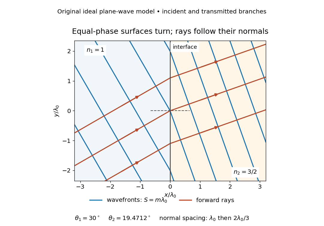
The diagram shows incident and transmitted branches separately, with the reflected branch omitted. Its stipulated refractive indices are and , and its incident angle is to the interface normal. At a stationary interface, the frequency and tangential wavevector agree on the two sides: Snell's law gives , hence . The wavefronts turn while their normal spacing decreases from to , where is the vacuum wavelength. More explicitly, with normal to the interface and tangential, take for and for . These functions agree at ; the drawn wavefronts are at with . This is an exact piecewise plane wave phase construction for the stipulated transparent media, not measured material data. [ref]
The normal-to-wavefront rule requires its assumptions. In a medium with anisotropy, the wavevector remains normal to a smooth wavefront, but the group velocity and energy flux need not follow it. [ref] Near a wave caustic, where multiple light rays meet, one smooth phase function may no longer describe the field; diffraction and the full wave amplitude matter. A wavefront is also not generally a surface of equal pulse arrival time. In a medium with optical dispersion, a monochromatic wave phase moves with the phase velocity, while a sufficiently narrow wave packet follows the group velocity. Even identical optical path lengths at one frequency can give different group delays. The usual equal-travel-time picture needs a common launch reference and a nondispersive ray model; an arbitrary broadband disturbance has no single monochromatic wavefront.[ref]
Wavefront curvature describes the change in the normal direction across a surface of equal wave phase. A plane wavefront has zero curvature; a spherical wavefront has curvature magnitude for radius . A general wavefront can have different principal curvatures in different transverse directions. The sign convention must be stated when distinguishing converging and diverging waves.[ref]
RP Photonics Encyclopedia by Rüdiger Paschotta. Wavefronts entry, wavefront shapes and changes produced by lenses
In a paraxial transverse plane, choose the convention in which a diverging spherical wave has . Its quadratic phase variation is approximatelyThe corresponding local ray angle is approximately . For illustrative and , the angle is radians and the optical path difference is . At wavelength , that is eight phase cycles. A modest geometrical departure can therefore produce a substantial optical phase difference.
For an ideal Gaussian beam with its waist at ,The reciprocal form remains finite at the waist: its value is zero, so the wavefront there is locally planar even though the beam radius is minimal. At , . Beam size and curvature are distinct beam parameters.[ref]
Propagation of a Gaussian Beam Through a Thin Lens by Francesco D'Angelo. Radius of Curvature of Gaussian Wavefronts, equation (6); complex parameter, equation (10)
A thin lens changes the curvature according to in this convention, while the beam radius at the lens is unchanged in the thin-element approximation.[ref] Thus a lens can alter convergence without an immediate jump in the beam width.
Experimentally, curvature can be inferred from a measured phase profile or local wavefront slopes. Phase unwrapping and the chosen reference matter because an intensity image in one plane does not itself provide the quadratic phase. A curved wavefront is not necessarily aberrated: the appropriate ideal reference can itself be spherical or Gaussian-beam curvature.
An optical path length measures how much propagation wave phase a path accumulates, expressed as the distance that would accumulate the same wave phase in vacuum. A centimetre in a uniform medium with refractive index has optical path length , although its geometric length remains . This makes optical path length useful whenever two contributions must arrive with matching wave phases, from an optical lens to a Michelson interferometer. [ref]
For a specified path at fixed angular frequency , the optical path length is the line integralHere is geometric arc length, and is the phase refractive index, evaluated at the same frequency everywhere. The propagation interpretation assumes a stationary linear medium with isotropy, a real positive scalar refractive index and negligible loss, on a valid geometrical optics branch. The path can curve; at sharp interfaces apply the appropriate matching conditions to each segment. A prescribed curve has a mathematical line integral, but it predicts a propagation wave phase only when it represents the physical branch. [ref] Optical fibers can require a mode wavenumber rather than the bulk refractive index along a guessed light ray. [ref]
Fix the vacuum wavelength , with frequency and vacuum wavenumber . In a locally uniform medium the wavelength is , while the frequency stays unchanged at a stationary interface. With the convention , propagation from a specified starting wave phase contributesThe relative reference includes launch wave phases and any extra wave phase from mirrors, beam splitters or coatings. Thus is a propagation contribution, not an absolute detector wave phase independent of the apparatus. If the reference contributions stay fixed, a change in optical path difference changes the phase difference by . Using the material wavelength again in this formula would count the refractive index twice. [ref]
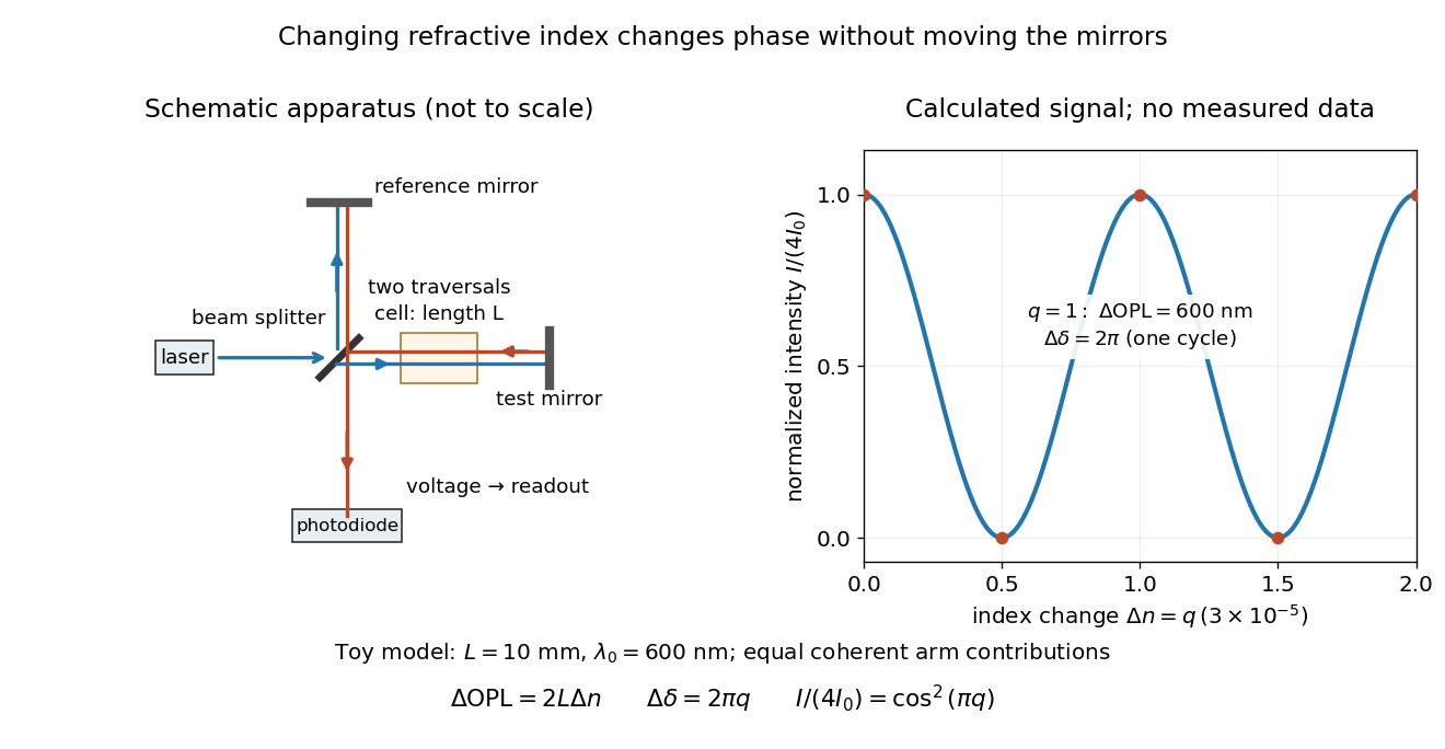
Optical path difference in a Michelson interferometer: apparatus schematic and a calculated phase difference readout
. Details. A motivating measurement turns invisible optical oscillations into a slowly changing electrical signal. MIT's teaching experiment uses a laser, a beam splitter, two returning mirrors, an amplified photodiode, an oscilloscope and a calibrated mirror actuator driven by a function generator. The returning beams overlap on the photodiode; one channel records detector voltage and another the actuator drive. The measured observable is the changing light intensity, including its maxima and minima, rather than direct timing of an optical cycle. A calibrated displacement per drive voltage and the spacing of the extrema relate geometric motion to the phase difference. The guide infers the laser wavelength from known actuator calibration; conversely, with independently known vacuum wavelength and ambient refractive index, the same relation calibrates mirror motion. These two unknowns cannot both be inferred from fringe spacing alone. [ref]
For a proposed change-of-medium measurement, keep the mirrors fixed and put a transparent cell of internal length in one arm. Compare its contents at refractive indices and , leaving its windows in place. At normal incidence the two traversals giveHere is the signed number of whole interference fringe cycles plus any resolved fractional cycle, counted continuously. A mirror displacement instead gives ; distinguish this double-pass factor from a single pass in a Mach-Zehnder interferometer. OpenStax's gas-cell worked example provides the same double-pass reasoning; it is a teaching calculation rather than a published measurement dataset.[ref]
An exact toy calculation makes the sensitivity visible. Stipulate , and . Then and : a full interference fringe cycle, despite unchanged geometric lengths. For a continuous change , let and choose the initial detector phase difference to be zero. Equal coherent detected arm contributions of light intensity predictThe plot is this stipulated model: gives a minimum, restores a maximum, and the reference level is chosen by adjustment of the apparatus. It contains no measured values or assigned properties of a real gas. The equivalent mirror travel in vacuum is per cycle. A single endpoint light intensity cannot distinguish from ; the continuous fringe count carries the missing information.
For an interpretable cell measurement, establish the initial phase difference with a small calibrated mirror scan, then track slow changes through successive interference fringes. Measure the dark signal and each arm separately, keep photodiode gain within its linear range, align both beams on the same region and match their linear polarizations. Monitor interferometric visibility and keep arm delays within the useful optical coherence time. Record cell length, contents, pressure and temperature; return to the starting condition to check drift. Changes in window deformation, cell length, external air or mirror position also change optical path length, so a reference cell or an independently monitored mechanical path is needed to isolate the contents' refractive index. These controls are deductions from the model, not a claim that the illustrated apparatus was operated. Loss of fringe count leaves a whole-cycle ambiguity; at an intensity extremum the first derivative with respect to phase difference vanishes, so a scan around phase quadrature is more sensitive to small changes. Broadband illumination, unstable optical coherence, vibration and strong loss can invalidate a simple one-frequency inference.
An optical path difference subtracts two optical path lengths at the same frequency and with specified endpoints and sign. Its phase difference contribution is , in addition to any apparatus reference wave phase. For wavefront error, the comparison is usually between an actual wavefront and an ideal reference wavefront.
In a monochromatic two-path interferometer, an ideal phase plate of thickness and refractive index adds phase at normal incidence. The interference pattern is unchanged when for integer , provided transmitted amplitudes and alignment are unchanged. Calling the smallest index requires specifying the admissible range; excludes the optically null solution.
The group refractive index is for a transparent isotropic propagation branch with forward group velocity . Differentiating the local wavenumber givesThe last formula gives the propagation group delay along a path whose geometry is fixed as frequency varies; additional apparatus wave phases require their own frequency derivatives. For a narrow wave packet with little loss and negligible reshaping, it approximates the transit of its wave envelope. In the nondispersive case , it reduces to . An optical path length at one frequency contains no information about , so in a medium with optical dispersion it cannot by itself determine the group delay. [ref]
For an original local model near , choose two equal geometric paths of length , with and . At both optical path lengths equal , and matched launch and interface references give equal carrier wave phases. But and , so their group delays differ by . This local stipulated model is a counterexample to identifying equal wave phase with equal pulse arrival; it asserts no material response outside the narrow band considered. Strong loss or pulse reshaping requires a fuller propagation model, and group delay need not time the earliest causal response.
For vacuum incidence at fixed angle into a transparent isotropic medium, Snell's law gives . Thus , andAngles must be differentiated in radians. This determines the local group velocity from a first derivative of measured refraction angles; pulse broadening needs further information about group velocity dispersion and absorption.
The group delay is the frequency derivative of an unwrapped transfer wave phase, using the convention. It predicts the leading delay of a narrow wave envelope when the transfer wave amplitude and the delay vary little across its band; it is not generally a signal-front arrival time.
The second derivative of spectral phase with respect to angular frequency; it measures variation of group delay with angular frequency.
The cubic term in a component's spectral phase, conventionally written , where is an angular frequency offset.
A wavefront error is the difference in optical path length from a reference wavefront, often an ideal plane or sphere. Its root mean square should specify the illuminated pupil and which modes, such as constant phase or image displacement, have been removed.
For a real wavefront error , its squared spatial root mean square is . Orthogonal unit-peak sine modes have mean square , so , whereas the coefficient norm is . On a finite optical pupil orthogonality needs checking; independent uniform random wave phases give the same diagonal after wave phase averaging. This normalization matters when a speckle contrast of a sinusoidal wavefront error is specified by peak wave amplitude.
Wave interference is the reinforcement or cancellation that occurs when overlapping wave amplitudes add by the superposition principle. For two monochromatic waves of the same frequency, mutual optical coherence means that their relative wave phase is stable during the observation. Equal wave phases give constructive interference; a half-cycle phase difference gives the destructive interference intensity minimum. Wave amplitudes add before their squares determine wave intensity. [ref]
https://openstax.org/books/university-physics-volume-3/pages/3-1-youngs-double-slit-interference. Ling, Sanny and Moebs, University Physics Volume 3, §3.1: coherent waves and interference
.Consider two overlapping beams in a homogeneous medium, with the same polarization of an electromagnetic wave and individual local time-averaged light intensities . Their phase difference is measured in radians. In the scalar detection convention, the combined local time-averaged wave intensity isThe last term records wave interference; adding alone misses it. The formula describes irradiance when both fields propagate along the same direction, or when the same detector geometry factor is included in all three intensities. For crossing beams it describes the squared electric field response, proportional to scalar wave intensity; a specified component of the Poynting vector also requires the propagation geometry. The ideal crossing plane waves below make that distinction explicit.
For equal individual light intensities , the cosine half-angle identity givesThe constructive interference intensity is at modulo , and the destructive interference intensity is zero at modulo . At phase quadrature, , it is . With and in the same arbitrary wave intensity unit, the maximum is , the minimum is , and the phase quadrature value is : unequal wave amplitudes cannot cancel completely.
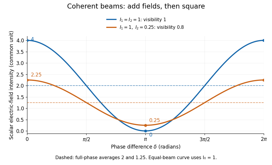
Two-beam wave intensity versus phase difference: equal beams reach 4 and 0; unequal beams reach 2.25 and 0.25
. Details. Both curves use the same wave intensity unit and a horizontal angle in radians. The dashed levels are the averages over a full phase difference cycle. Equal beams have interferometric visibility one; the unequal example has interferometric visibility .
A spatially varying phase difference turns the same law into interference fringes. Take two ideal plane electromagnetic waves with common wavelength , equal individual light intensities , and propagation directions at angles and from the axis in the plane, with . Both have linear polarization along , perpendicular to both propagation directions. Choose equal initial wave phases; their wavevectors and phase difference areHere is the wavenumber and the angular frequency. The common and time terms cancel, so the interference fringes stay at fixed for every . Their interference fringe spacing isSet the length unit to , so that , and take : then . The constructive interference intensity bands lie at integer ; the destructive interference intensity bands lie at half-integer .
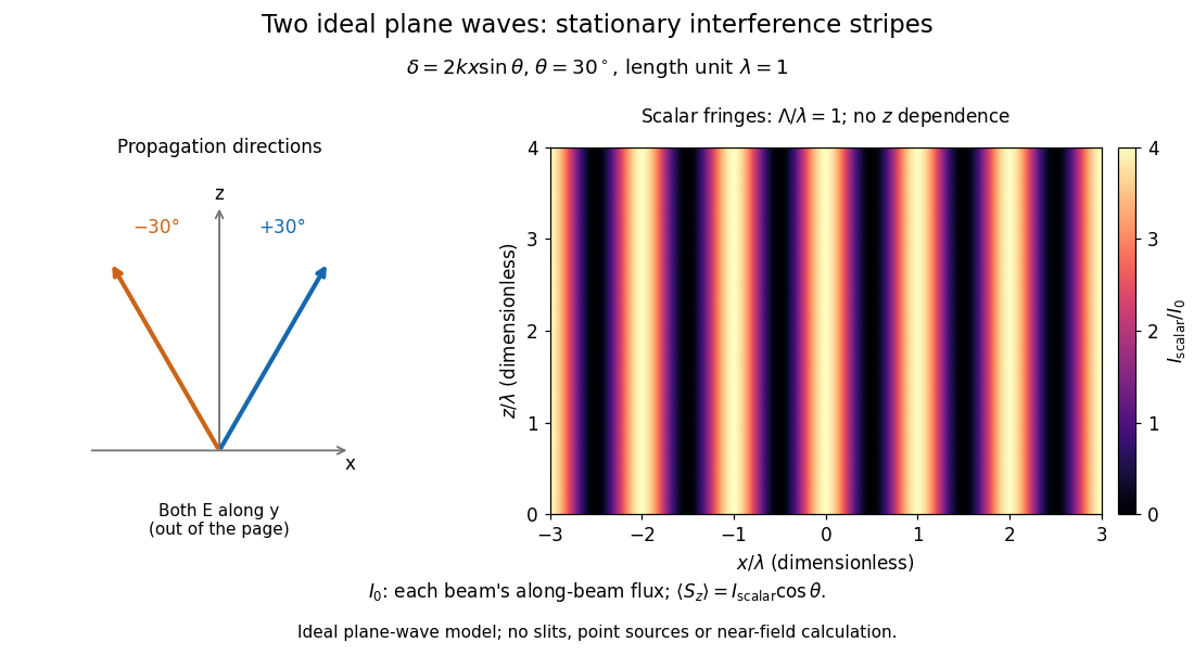
The grid covers and ; both axes are dimensionless lengths in wavelength units. The colour scale is from zero to four, using the same single-beam normalization as the equal-beam curve above. This is an ideal plane wave superposition, with no slits or point sources and no near-field approximation. For these -polarized plane electromagnetic waves in vacuum, the longitudinal time-averaged Poynting vector obeys ; the plotted scalar therefore differs from the irradiance through a plane normal to by that common factor. This relation follows by adding the magnetic fields as well as the electric fields.
The bright peaks do not create energy. Averaging over one interference fringe spacing, or equivalently over one full phase difference cycle, givesbecause the integral of the cosine is zero, with sine as its antiderivative. Equal beams thus average to , despite bright bands at . For the crossing-wave geometry, the average longitudinal energy flux is correspondingly . Bright and dark regions redistribute the incoming energy; conservation of energy concerns the full energy flux, rather than the height of one peak.
Wave interference is useful because phase differences convert small changes in optical path length into measurable changes of wave intensity, as in a Mach-Zehnder interferometer. Its beauty is that the same superposition principle produces both complete cancellation and fourfold brightening; adding more coherent contributions also produces the narrow peaks of a diffraction grating. Feynman's treatment connects this many-source pattern directly to addition of complex amplitudes. [ref].
A short proof outline uses local real fields with parallel linear polarizations. Write and for the same positive conversion factor . Averaging over many wave periods while the phase difference stays fixed uses and , giving the stated law. Equivalently, add the complex amplitudes and take the squared complex modulus. [ref]
https://www.feynmanlectures.caltech.edu/I_29.html#Ch29-S5. Feynman, Leighton and Sands, The Feynman Lectures on Physics, I §29–5: the mathematics of interference
.For different fixed linear polarizations in a common transverse plane, the cross term acquires the dot product of their real unit vectors, equal to for relative angle . Orthogonal linear polarizations remove the cross term in polarization-insensitive scalar detection; different orientations generally only reduce it. A common polarizer can select overlapping components and recover wave interference. Likewise, rapid random variation of the phase difference removes the observed cross term only when the detector's time average has . Slowly varying wave phases can instead move resolved interference fringes, and biased or incompletely sampled wave phases can leave residual contrast. Finite optical coherence therefore depends on the observation time as well as the fields.
Lloyd's mirror produces interference between light arriving directly from a narrow source and light reflected by a plane mirror, which appears to originate at the source's virtual image. With source distance from the mirror, the effective source separation is . A reflection phase shift close to reverses the bright/dark condition relative to two equally phased sources. Spatial filtering, suitable temporal coherence, and direct/reflected beam overlap remain necessary.
Measurement using wave interference: relative path or phase changes are inferred from the resulting signal. The interacting fields must have sufficient optical coherence in the measured modes for the intended interference signal.
Phase unwrapping reconstructs a wave phase field from measurements that determine only its value modulo . If a detector or complex-argument calculation returns , then all values with integers give the same wrapped observation. Recovering a continuous wave phase therefore requires information beyond each isolated value. A primary 1982 analysis discusses this problem in wave phase curves obtained from image Fourier transforms before averaging them.[ref]
Analysis of the phase unwrapping algorithm by Kazuyoshi Itoh. Primary abstract, phase ambiguities and tracking motivation
Define with principal interval . If adjacent true differences satisfy , thenStarting from one reference wave phase, adding these wrapped differences reconstructs the sampled wave phase up to a global multiple of . The proof is direct: wrapping the two endpoint phases changes their difference only by an integer multiple of , and the strict bound selects its unique representative.
For an original example, true phases wrap to . Their wrapped increments are all , so reconstruction succeeds. But true increments produce exactly the same wrapped samples as increments . No algorithm can distinguish those two possibilities from the samples alone without a further assumption. Increasing sampling density can restore the bound only when the field's variation and noise allow it.
In two dimensions, different integration paths introduce a consistency test. A nonzero integer multiple of in the sum of wrapped increments around a closed sampling loop is a phase-unwrapping residue. Noise, undersampling or true wave phase singularities can obstruct a single consistent smooth reconstruction. Choosing an integration path is therefore part of the inference.
For interferometry, low interference visibility can make the wave phase poorly determined even before unwrapping. Unwrapping does not recover information lost where the measured complex amplitude vanishes, nor does it distinguish an actual discontinuity from a smooth but insufficiently sampled change. Report the wave phase reference, principal interval, sampling and any continuity assumptions alongside the reconstructed field.
Phase-shifting interferometry measures an optical phase difference by recording light intensities at controlled relative wave phase shifts. For two sufficiently coherent fields at one detector point, a common model iswhere is a common background, a modulation amplitude and a known applied step. Several measurements separate the unknown wave phase from light intensity background and contrast; a single bright or dark frame generally cannot do so.
A concrete primary implementation was reported in 1974. A piezoelectrically varied reference arm and a 1024-element photodiode array supplied sampled light intensities to a minicomputer, which recovered wave phase by synchronous Fourier-series detection. The paper describes optical-surface and lens testing, repeated sampling and compensation of instrumental wavefront errors.[ref]
Digital Wavefront Measuring Interferometer for Testing Optical Surfaces and Lenses by J. H. Bruning and others. Abstract and p. 2693, apparatus and phase-detection method
This is an experimental implementation of controlled wave phase modulation; it is not a claim that every such system uses the same number of steps.Writing the model asturns wave phase recovery into a linear fit followed by . The step choices must make the three columns independent. Repeating only the same wave phase cannot identify all three unknowns. With more steps, least squares can fit the coefficients while exposing model residuals.
A reflecting reference mirror moved axially by changes its round-trip optical path by in the simple normal-incidence geometry, giving . A quarter-cycle wave phase step thus corresponds to ; at 632.8 nm this is 79.1 nm. These are geometric model values, not a calibration result for the historical apparatus.
Phase-step calibration error, light intensity drift, motion between frames and detector nonlinearity can all break the common-intensity model. The retrieved wave phase remains modulo , so phase unwrapping requires additional spatial or temporal information. The useful observable is the relative wave phase under controlled acquisition conditions, not an absolute optical wave phase inferred from brightness alone.
Four-step phase retrieval estimates relative wave phase from four wave interference frames separated by quarter-cycle wave phase steps. Use the explicit signal-arm conventionwith a common background and modulation amplitude . Opposite-frame differences giveso . The order of the subtractions fixes the sign. Changing which arm receives the wave phase step requires a correspondingly changed convention.
The same data estimate and . A simple model-consistency residual is , which is zero for the exact stated model. It does not detect every possible systematic error.
For an original example, let , and . The four light intensities are , , and . Then , , and the recovered wave phase is . Common background cancels, whereas changing background separately between frames need not cancel.
If independent additive errors in the four light intensities have common variance , first-order propagation givesThis follows from and difference variances . It applies away from vanishing modulation and assumes the specified independent equal-noise model. wave phase uncertainty grows when interference visibility is weak.
The method is a discrete instance of phase-shifting interferometry, whose early digital apparatus used controlled reference-path modulation and synchronous wave phase extraction.[ref]
Digital Wavefront Measuring Interferometer for Testing Optical Surfaces and Lenses by J. H. Bruning and others. Abstract, reference-arm modulation and Fourier-series detection; the four-frame derivation here is separate
The result is still a principal wave phase; phase unwrapping cannot be replaced by choosing a different arctangent branch at each pixel without a consistency rule.Intensity interferometry infers source coherence from correlations between measured intensities, rather than directly combining electric-field amplitudes. For stationary chaotic Gaussian light, the normalized correlations satisfy , under the relevant statistical assumptions.
Separated detectors can therefore measure the magnitude of spatial coherence, which is related to the source's angular structure. Optical carrier phase need not be stabilized as in amplitude interferometry, but fast timing and sufficient photon statistics are crucial. The squared magnitude does not by itself retain every phase needed for unrestricted image reconstruction.
Measurement using interfering light fields. A phase difference changes the detected intensity, allowing measurements of displacement, optical path length or a spectrum. The round-trip phase in a Michelson interferometer gives one explicit path-to-phase calibration; Fourier transform spectroscopy recovers spectral information from an interferogram.
A nearly uniform wavefront phase over one collector is called its piston. Differential atmospheric piston changes the pairwise optical phase without requiring a change in the source. Delay tracking and closure phase address different consequences of this phase error; intensity correlations are unchanged by an ideal pure phase multiplication at either detector.
fringe tracking estimates changing optical delay or phase and adjusts delay compensation to keep an astronomical interferometer near a useful interference condition. The delay must first lie inside the finite-bandwidth coherence envelope; rapid tracking then controls atmospheric piston. This is optical-path stabilization, with sensitivity and reference-source limitations.
A Moiré pattern is a large-scale modulation produced by superposing similar periodic structures. Two identical two-dimensional lattices rotated by a small angle have geometric period in the usual matching geometry. In layered crystals this modulation can act as an electronic superlattice; the actual bands additionally depend on interlayer coupling and orbital structure.
A slow spatial modulation produced by overlapping periodic structures with different projected spatial frequencies or orientations. Its spacing need not equal an atomic lattice spacing.
Subtract the phases and of two projected periodic structures. Their relative phase repeats along the difference vector after distance . For magnitudes and separated by angle , this gives . At zero rotation it reduces to ; equal spacings give . Finite specimen extent limits how many periods can be observed.
Destructive interference occurs when coherent contributions partially or completely cancel their complex amplitudes. For two equal contributions, a phase difference of modulo gives zero resultant wave amplitude. The missing local light intensity is consistent with conservation of energy because the full spatial interference pattern redistributes power.
Thin-film interference combines coherent light contributions reflected or transmitted at the two surfaces of a layer. For a film of refractive index , thickness and internal angle , the round-trip optical path difference is . The relative reflection phase shift must also be included. For a nonabsorbing higher-index film surrounded by air, one of the two leading reflected contributions has a phase shift and the other does not. Reflection maxima therefore satisfy . A smooth reflection spectrum filters many visible wavelengths at once; varying thickness and angle produce spatially varying mixed colours.
A thin liquid layer whose two reflected beams can interfere. For air on both sides, one surface reflection has a phase reversal; a constructive reflected condition is . Thickness and viewing angle therefore alter the selected colours.
With one reflection phase reversal and near-normal incidence, reflected minima satisfy . Subtracting the reciprocal-wavelength conditions for consecutive minima gives the displayed thickness relation. A single maximum between two stated minima identifies the consecutive-order case. Wavelength-dependent refractive index or non-air surroundings can change the inference.
An optical coating designed to reduce reflection through refractive-index choice and thin-film interference. A quarter-wave design is a single-wavelength approximation, not broadband perfection.
Articles were limited to the first 100 out of 289 total.
Articles by others on the same topic



Physical optics is a branch of optics that focuses on the wave nature of light and its interactions with matter. Unlike geometrical optics, which primarily deals with the propagation of light in terms of rays and prisms, physical optics examines phenomena such as interference, diffraction, and polarization, which cannot be adequately explained by ray optics alone. Key concepts in physical optics include: 1. **Wave Nature of Light**: Light is treated as a wave, which means it is subject to wave phenomena.